- Home
- :
- All Communities
- :
- User Groups
- :
- Enterprise Spatial Analytics
- :
- Blog
- :
- Esri and Snowflake Series: Protecting Lives & Infr...
Esri and Snowflake Series: Protecting Lives & Infrastructure from Wildfires using Telco Data
- Subscribe to RSS Feed
- Mark as New
- Mark as Read
- Bookmark
- Subscribe
- Printer Friendly Page
In this first installment of our blog series on Enterprise Spatial Analytics, we dive into one of the most potent yet underused features in ArcGIS Pro: Query Layers.
As organizations increasingly migrate their data infrastructure to modern cloud platforms like Snowflake, the ability to perform spatial analytics without moving or duplicating data becomes essential. This series will walk through how Esri’s ArcGIS platform integrates natively with cloud data warehouses, enabling real-time spatial intelligence at scale.
We’ll begin by exploring how ArcGIS Pro connects directly to Snowflake using query layers—allowing analysts and GIS professionals to build dynamic maps, perform spatial queries, and aggregate data using SQL—all without leaving the ArcGIS environment or replicating data.
In future posts, we’ll extend this workflow to:
- Perform GeoAI analysis with deep learning models and Sentinel-2 imagery – Part 2
- Use ArcGIS Data Interoperability to read and write data into Snowflake – Part 3
- Utilize map-centric apps and ArcGIS Data Pipelines to deliver actionable insights to business users and emergency responders – Part 4
Whether you’re a data engineer, GIS analyst, or public safety decision-maker, this series will help you unlock the full power of analytics by combining Esri and Snowflake. So let’s start creating our Query Layers.
Note: To complete this segment, you need to download CALIFORNIA_ADDRESSES and CELL_TOWERS_WITH_RISK_SCORE tables from this link. Then create a new Database named Esri_HOL and load these tables into the Public Schema in Snowflake.
Step 1: Connecting ArcGIS Pro to Snowflake
Open your ArcGIS Pro project and follow these steps to set up a live connection to Snowflake.
Open the Catalog Pane
Right-click on Databases, then select New Database Connection.
For Database Platform, choose Snowflake.
Provide the full server name, which includes .snowflakecomputing.com.
Select your Authentication Method and enter your credentials.
Fill in the Role, Database, Schema, and Warehouse.
✅This connection does not require any data replication. ArcGIS Pro pushes SQL queries directly to Snowflake and displays the data returned, making it ideal for working with large datasets.
Once connected, you’ll be able to explore your Snowflake schema and see which tables are spatial and which are non-spatial.
Step 2: Creating a Query Layer for Customer Addresses
We’ll start by visualizing customer address data stored in Snowflake.
In the Command Search Box, type Query Layer.
Click Query Layer, and select your Snowflake connection.
Enable the List Tables checkbox and select ADDRESSES table.
ArcGIS auto-generates a SQL query, you can add the LIMIT 100: SELECT * FROM CALIFORNIA_ADDRESSES LIMIT 100. This retrieves a sample of 100 records.
Click next
💡 Tip: You can optionally check the box “Create materialized view on output”.
When enabled, ArcGIS will store the output of your query layer as a materialized view in Snowflake.
Why it matters: In Esri workflows, this improves performance for frequently accessed or complex layers (especially with joins or spatial filters). It reduces load time in maps or dashboards and minimizes repeated query processing against large datasets.
Set the unique identifier field (e.g., ADDRESS_ID)
Choose Point as the geometry type
This query layer now dynamically fetches Snowflake data and renders it on your map as a spatial layer—without duplication.
As the result is shown in the map , zoom in into the layer.
Step 3: Filtering Query Layer by City
Next, let’s zoom in on a specific city—Malibu.
Edit your query layer using the Edit Query tool. To the command box and type edit query layer.
Replace the SQL with:
FROM DEFAULT_DATABASE.DEFAULT_SCHEMA.CALIFORNIA_ADDRESSES WHERE city = 'Malibu'

This modified layer now only displays customer data for Malibu. Query layers push the SQL logic directly to Snowflake, ensuring minimal latency and maximum performance.
Step 4: Aggregating Data Using H3 Spatial Functions
To analyze density, we’ll aggregate customers into hexagonal bins using H3 geospatial functions (available in Snowflake).
Create a new Query Layer, select the Table CALIFORNIA_ADDRESSES and enter this:
H3_POINT_TO_CELL("GEOG", 4) AS h3_id,
COUNT(*) AS pt_count,
H3_CELL_TO_BOUNDARY(h3_id) AS h3_geo
FROM
DEFAULT_DATABASE.DEFAULT_SCHEMA.ADDRESSES GROUP BY
h3_id
Explanation:
H3_POINT_TO_CELL maps a point to a hexagon at resolution 4.
COUNT(*) counts how many customers fall in each bin.
H3_CELL_TO_BOUNDARY returns the polygon geometry for each hex bin.
Set:
h3_id as the unique ID
Geometry type as Polygon
ArcGIS will take the geometries and render the aggregated map
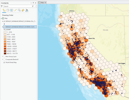
Now you’ve created an aggregated density layer driven directly by Snowflake and powered by spatial SQL. Use Graduated Colors symbology to visually identify hotspots.
From the Contents pane, right-click on the layer and choose Symbology.
Here, you will allow the count of the points in each bin, to be used to drive the colors.
- Select Graduated Colors.
- Select 10 classes.
- Select the PT_Count as the Field.
Step 5: Adding Cell Tower Data
To bring in telco infrastructure:
In the Catalog Pane, under your Snowflake connection, right-click on CELL_TOWERS_WITH_RISK_SCORE.
Click Add to Current Map
Use CELL_ID as the unique identifier.
Set geometry type to Point.
Now your map shows both customer clusters and cell tower locations, opening the door to GeoAI-based vulnerability assessments.
To Summarize
ArcGIS Pro’s query layers are a game-changer when working with cloud data warehouses including Snowflake, Google BigQuery, and Amazon Redshift. You can:
Perform real-time analysis without ETL or data duplication
Push heavy spatial workloads to powerful compute engines
Create seamless visualizations that reflect up-to-date cloud data
This workflow is part of a broader effort to unlock disaster resilience with spatial intelligence, bridging cloud-scale data engineering and mission-critical geospatial analysis.
Stay tuned for the next blog in this series where we’ll apply deep learning, STAC, and ArcGIS Online to complete the GeoAI pipeline!
You must be a registered user to add a comment. If you've already registered, sign in. Otherwise, register and sign in.


