Python Blog - Page 4

Buffering

Probably one of the first things you did in a GIS class.

Select all the fast food outlets that are within 1 mile/km of a school. 

To the rescue... a little buffer, a selectorama, intersect, spatial join... whatever.  At some stage you have used buffers for spatial delineation either by creating one as a feature layer, or virtually when you select things within-a-distance-of.

So initially I thought I would just show the geometry created by buffering a simple shape or two to show the point densification on the outward corners.  In the old days a buffer around a point was represented by a 36-sided circle, if you like, an n-gon.  Pretty good if the buffer was small, but seriously lame when the buffer radius was very large.  Crrrrankout a buffer on a shapefile to see what I mean.  Many a line of code was written to approximate a true circle.  Now you can.

But what about a buffer?  The outward corners have that circular appearance, maintaining the offset radius (aka the buffer size) from the line work.  One would expect teeny-tiny circular arcs to appear in the geometry representation.  At worse, perhaps an n-gon representation of the arc.

Not so.  Here is a square green polygon being shown in Spyder with the arcpy's new svg display.  Pretty cool, but I like my numpy array version better (in red)

p_0[0]
<Array
 [<Point (300010.0, 5000000.0, #, #)>,
  <Point (300010.0, 5000010.0, #, #)>,
  <Point (300020.0, 5000010.0, #, #)>,
  <Point (300020.0, 5000000.0, #, #)>,
  <Point (300010.0, 5000000.0, #, #)>]>‍‍‍‍‍‍‍‍‍‍‍‍‍‍‍‍‍‍‍‍‍‍‍‍‍‍‍‍‍‍‍‍‍‍‍‍‍‍‍‍‍‍‍‍‍‍‍‍‍‍‍‍‍‍‍‍‍‍‍‍‍‍‍‍‍‍‍‍‍‍‍‍‍‍‍‍‍‍‍‍‍‍‍‍‍‍‍‍‍‍‍‍‍‍‍‍‍‍‍‍‍‍‍‍‍

coords = [(i.X - 300000, i.Y - 5000000)
           for i in p_0[0]]

coords
[(10.0, 0.0),
 (10.0, 10.0),
 (20.0, 10.0),
 (20.0, 0.0),
 (10.0, 0.0)]‍‍‍‍‍‍‍‍‍‍‍‍‍‍‍‍‍‍‍‍‍‍‍‍‍‍‍‍‍‍‍‍‍‍‍‍‍‍‍‍‍‍‍‍‍‍‍‍‍‍‍‍‍‍‍‍‍‍‍‍‍‍‍‍‍‍‍‍‍‍‍‍‍‍‍‍‍‍‍‍‍‍‍‍‍‍‍‍‍‍‍‍‍‍‍‍‍‍‍‍‍‍‍‍‍‍‍‍‍‍‍‍‍‍‍‍‍‍‍‍‍‍‍‍‍‍‍‍‍‍‍‍‍‍

p0
Geo([[10., 0.],
     [10., 10.],
     [20., 10.],
     [20., 0.],
     [10., 0.]])‍‍‍‍‍‍‍‍‍‍‍‍‍‍‍‍‍‍‍‍‍‍‍‍‍‍‍‍‍‍‍‍‍‍‍‍‍‍‍‍‍‍‍‍‍‍‍‍‍‍‍‍‍‍‍‍‍‍‍‍‍‍‍‍‍‍‍‍‍‍‍‍‍‍‍‍‍‍‍‍‍‍‍‍‍‍‍‍‍‍‍

In both cases, the coordinates are held in an array of some kind as in the above. 

In the example p_0 is the arcpy.Polygon and p_0[0] is the slice of the first object within... an arcpy.Array of arcpy.Point objects.

So what do the buffer coordinates look like?

b_0 = p_0.buffer(1)
b_0[0] # get the array
<Array
 [<Point (300020.0449000001, 4999999.001, #, #)>,
 <Point (300020.0, 4999999.0, #, #)>,
 <Point (300010.0449000001, 4999999.000499999, #, #)>,
 <Point (300010.0, 4999999.000600001, #, #)>,
 <Point (300009.0, 5000000.0, #, #)>,
 <Point (300009.0, 5000010.0, #, #)>,
 <Point (300010.0, 5000011.0, #, #)>,
 <Point (300020.0, 5000011.0, #, #)>,
 <Point (300021.0, 5000010.0, #, #)>,
 <Point (300021.0, 5000000.0, #, #)>,
 <Point (300020.0449000001, 4999999.001, #, #)>]>‍‍‍‍‍‍‍‍‍‍‍‍‍‍‍‍‍‍‍‍‍‍‍‍‍‍‍‍‍‍‍‍‍‍‍‍‍‍‍‍‍‍‍‍‍‍‍‍‍‍‍‍‍‍‍‍‍‍‍‍‍‍‍‍‍‍‍‍‍‍‍‍‍‍‍‍‍‍‍‍‍‍‍‍‍‍‍‍‍‍‍‍‍‍‍‍‍‍‍‍‍‍‍‍‍‍‍‍‍‍‍‍‍‍‍‍‍‍‍‍‍‍‍‍‍‍‍‍‍‍‍‍‍‍‍‍‍‍‍‍‍‍‍‍‍‍‍‍‍‍‍‍‍‍‍‍‍‍‍‍‍‍‍‍‍‍‍‍

b_0.__geo_interface__
{'type': 'MultiPolygon',
 'coordinates':
 [[[(300020.0449000001, 4999999.001),
    (300020.0, 4999999.0),
	(300010.0449000001, 4999999.000499999),
	(300010.0, 4999999.000600001),
	(300009.0, 5000000.0),
	(300009.0, 5000010.0),
	(300010.0, 5000011.0),
	(300020.0, 5000011.0),
	(300021.0, 5000010.0),
	(300021.0, 5000000.0),
	(300020.0449000001, 4999999.001)]]]}‍‍‍‍‍‍‍‍‍‍‍‍‍‍‍‍‍‍‍‍‍‍‍‍‍‍‍‍‍‍‍‍‍‍‍‍‍‍‍‍‍‍‍‍‍‍‍‍‍‍‍‍‍‍‍‍‍‍‍‍‍‍‍‍‍‍‍‍‍‍‍‍‍‍‍‍‍‍‍‍‍‍‍‍‍‍‍‍‍‍‍‍‍‍‍‍‍‍‍‍‍‍‍‍‍‍‍‍‍‍‍‍‍‍‍‍‍‍‍‍‍‍‍‍‍‍‍‍‍‍‍‍‍‍‍‍‍‍‍‍‍‍‍‍‍‍‍‍‍‍‍‍‍‍

b_0.JSON
'{"curveRings":
  [[[300020.0449000001,4999999.0010000002],
    [300020,4999999],
    [300010.0449000001,4999999.0004999992],
    [300010,4999999.0006000008],
 {"c":[ [300009,5000000],
      [300009.29277758137,4999999.2929531736]]},
      [300009,5000010],
 {"c":[[300010,5000011],
       [300009.29287232383,5000010.7071276763]]},
      [300020,5000011],
 {"c":[[300021,5000010],
       [300020.70712767617,5000010.7071276763]]},
      [300021,5000000],
{"c":[[300020.0449000001,4999999.0010000002],
      [300020.72280301224,4999999.3089512894]]}]],
 "spatialReference":{"wkid":2146,"latestWkid":2951}}'‍‍‍‍‍‍‍‍‍‍‍‍‍‍‍‍‍‍‍‍‍‍‍‍‍‍‍‍‍‍‍‍‍‍‍‍‍‍‍‍‍‍‍‍‍‍‍‍‍‍‍‍‍‍‍‍‍‍‍‍‍‍‍‍‍‍‍‍‍‍‍‍‍‍‍‍‍‍‍‍‍‍‍‍‍‍‍‍‍‍‍‍‍‍‍‍‍‍‍‍‍‍‍‍‍‍‍‍‍‍‍‍‍‍‍‍‍‍‍‍‍‍‍‍‍‍‍‍‍‍‍‍‍‍‍‍‍‍‍‍‍‍‍‍‍‍‍‍‍‍‍‍‍‍‍‍‍

b_0svg = b_0.__getSVG__()

b_0svg
'<path fill-rule="evenodd"
 fill="#66cc99" stroke="#555555"
 stroke-width="2.0" opacity="0.6" 
d=" 
M 300020.0449000001,4999999.001
 L 300020,4999999
  L 300010.0449000001,4999999.000499999
... snip
 L 300009,5000000
 L 300009,5000010
 L 300009.0048088113,5000010.098019366
... snip
 L 300010,5000011
 L 300020,5000011
 L 300020.09801936575,5000010.9951911885
...snip
 L 300021,5000010
 L 300021,5000000
 L 300020.9954546047,4999999.904777056
... snip
 L 300020.0449000001,4999999.001 z" />'
 

# ---- now take the same corner as an array

svg_arr
print(arc)                   ID    degrees 
[[20.        , 11.        ],   0
 [20.09801937, 10.99519119],   1
 [20.19509527, 10.98079709],   2    78.75
 [20.29029264, 10.95695635],   3
 [20.38269452, 10.92389861],   4    67.5
 [20.47141085, 10.8819423 ],   5
 [20.55558711, 10.83149154],   6    56.3
 [20.63441247, 10.7730323 ],   7
 [20.70712768, 10.70712768],   8    45.0
 [20.7730323 , 10.63441247],   9
 [20.83149154, 10.55558711],  10
 [20.8819423 , 10.47141085],  11
 [20.92389861, 10.38269452],  12
 [20.95695635, 10.29029264],  13
 [20.98079709, 10.19509527],  14    11.25
 [20.99519119, 10.09801937],  15
 [21.        , 10.        ]]) 16‍‍‍‍‍‍‍‍‍‍‍‍‍‍‍‍‍‍‍‍‍‍‍‍‍‍‍‍‍‍‍‍‍‍‍‍‍‍‍‍‍‍‍‍‍‍‍‍‍‍‍‍‍‍‍‍‍‍‍‍‍‍‍‍‍‍‍‍‍‍‍‍‍‍‍‍‍‍‍‍‍‍‍‍‍‍‍‍‍‍‍‍‍‍‍‍‍‍‍‍‍‍‍‍‍‍‍‍‍‍‍‍‍‍‍‍‍‍‍‍‍‍‍‍‍‍‍‍‍‍‍‍‍‍‍‍‍‍‍‍‍‍‍‍‍‍‍‍‍‍‍‍‍‍‍‍‍‍‍‍‍‍‍‍‍‍‍‍‍‍‍‍‍‍‍‍‍‍‍‍‍‍‍‍‍‍‍‍‍‍‍‍‍‍‍‍‍‍‍‍‍‍‍‍‍‍‍‍‍‍‍‍‍‍‍‍‍‍‍‍‍‍‍‍‍‍‍‍‍‍‍‍‍‍‍‍‍‍‍‍‍‍‍‍‍‍‍‍‍‍‍‍‍‍‍‍‍‍‍‍‍‍‍‍‍‍‍‍‍‍‍‍‍‍‍‍‍‍‍‍‍‍‍‍‍‍‍‍‍‍‍‍‍‍‍‍‍‍‍‍‍‍‍‍‍‍‍‍‍‍‍‍‍‍‍‍‍‍‍‍‍‍‍‍‍‍‍‍‍‍‍‍‍‍‍‍‍‍‍‍‍‍‍‍‍‍‍‍‍‍‍‍‍‍‍‍‍‍‍‍‍‍‍‍‍‍‍‍‍‍‍‍‍‍

So, What do the corners look like

As expected.  I created the rounded corners for the numpy-based Geo array.  In the example below, I plotted the SVG corner points and the Geo array points.  An angle of about 5 degrees (give or take) is used by both.  Smooth enough and you can account for area calculations if you know number of outward buffer corners, the total angular passage and the number n-gon shape.  Or just use arcpy's Polygon methods to get the area.

To leave you with some final thoughts. 

You can buffer 

• with a uniform distance around the shape
• an offset buffer, where the shape is expanded parallel to the forming lines (see above)
• a chordal buffer, (Buffer Geometry figure)
• buffer by increasing the area or perimeter (for polygons obviously).

This is an example of the last which is based on the offset buffer, but using area as the parameter.

So remember what goes into the buffer and that not all information that you would expect to see is shown in all forms of geometry representation.

Geometry ...

• 
   target="_self">Start with geometry
• SVG
• On to the Display
• Saving the SVG
• The Code

Previously...

/blogs/dan_patterson/2019/11/18/arcpy-shapes-viewing-in-spyder 

I really think it is a bit of overkill to create a FeatureClass just to see some geometry I have created or changed.

As of ArcGIS Pro 2.5, you can view a geometry object inside of Jupyter notebooks, Jupyter-lab or any other thing that supports SVG.  This missive shows how to view geometry from arcpy and also how to deal with geometry without having to go to arcpy to do it.

If you don't create or edit geometry with python, you can go now.

Start with geometry

Begin with some polygons.

In [ 1]: polys
In [or]: print(polys)
In [or]: polys.__repr__()

Out[1]:
[<Polygon object at 0x25941289d30[0x2594152f288]>,<Polygon object at 0x25941289cf8[0x259414a4bc0]>,
<Polygon object at 0x25941289c88[0x259414a4b98]>,<Polygon object at 0x25941289cc0[0x25940a241c0]>,
<Polygon object at 0x25941289c18[0x25940a240d0]>]

As In [ 1]: shows, you can get a 'representation' of the python geometry from within python.  It tells you that it is a polygon and then gives you the memory stuff (I presume).  The former you probably already knew and the latter you probably don't care about.  Pretty useless. So the quest continues.

Every object in python has a string representation, so lets try there.

In [ 2]: str(p_0)
In [or]: p_0.__str__()

Out[2]:
'<geoprocessing describe geometry object object at 0x000002594152F288>'

Heart be still! In [ 2]: is even more cryptic, but the memory location idea was spot on.

Let's see what 'dir' reveals.  I have snipped out a lot of stuff, and highlighted the more useful formats.  Make sure you explore the various geometry classes on your own.

In [3]: dir(p_0)

Out[3]:
['JSON', 'WKB', 'WKT', ... snip ...'__geo_interface__',
'__getSVG__', ... the new addition ....snip ...
'_fromGeoJson', ... snip ... '_repr_svg_', ... snip ...
...all the other properties and methods
]

Interesting.. maybe if a geometry contains more than one thing, slicing might real more.

In [4]: p_0[0]

Out[4]:
<Array
    [<Point (300010.0, 5000010.0, #, #)>, <Point (300010.0, 5000000.0, #, #)>,
    ... snip ...
    None,
          ... snip ...
    <Point (300002.0, 5000008.0, #, #)>, <Point (300001.0, 5000009.0, #, #)>,
    <Point (300001.0, 5000008.0, #, #)>, <Point (300002.0, 5000008.0, #, #)>]>

Perfect!  Polygons are made up of Array objects which are made up of Point objects.  Parts of arrays are separated by None, so you can have the polygons with multiple parts and/or holes in the parts.

Your education has been confirmed.

SVG

What is that __getSVG__ thing?

In [5]: p_0.__getSVG__()

Out[5]:
'<path fill-rule="evenodd"
fill="#66cc99"
stroke="#555555"
stroke-width="2.0"
opacity="0.6"
d=" M 300010,5000010 L 300010,5000000 L 300001.5,5000001.5 L 300000,5000010 L 300010,5000010
    M 300003,5000009 L 300003,5000003 L 300009,5000003 L 300009,5000009 L 300003,5000009
    M 300002,5000007 L 300001,5000007 L 300002,5000005 L 300002,5000007
    M 300002,5000008 L 300001,5000009 L 300001,5000008 L 300002,5000008
z"
/>'

Well they sure look like coordinates.  Time to go off and research SVG construction.

since __repr__ was revealing perhaps _repr_svg_ will be too.

In [6]: p_0._repr_svg_()

Out[6]:
'<svg xmlns="http://www.w3.org/2000/svg"
xmlns:xlink="http://www.w3.org/1999/xlink"
width="100.0" height="100.0"
viewBox="299999.6 4999999.6 10.800000000046566 10.800000000745058"
preserveAspectRatio="xMinYMin meet">
<g transform="matrix(1,0,0,-1,0,10000010.0)">
<path fill-rule="evenodd"
fill="#66cc99"
stroke="#555555"
stroke-width="0.21600000001490116"
opacity="0.6"
d=" M 300010,5000010 L 300010,5000000 L 300001.5,5000001.5 L 300000,5000010 L 300010,5000010
    M 300003,5000009 L 300003,5000003 L 300009,5000003 L 300009,5000009 L 300003,5000009
    M 300002,5000007 L 300001,5000007 L 300002,5000005 L 300002,5000007
    M 300002,5000008 L 300001,5000009 L 300001,5000008 L 300002,5000008
z"
/>
</g></svg>'

On to the Display

 Inside of Spyder, which uses an IPython console,

I used my handy function for representing a numpy-based array as geometry... which I was working with. 

You get a quick peek at what it looks like. 

The alternative???

•  use my other handy functions and make a featureclass,
• crank up Pro and
• add it to a map

Saving the SVG

Pretty easy.  Just right-click on it and you can save the SVG as an image or a *.svg file for use in such programs as Word.

The Code

I put it in a gist at...

 svg display for numpy geometries

If you are interested in alternatives and/or supplements to the various geometry packages, I have been working on

 ... npGeom ... which provides the basis for my

... Free Tools ...collection of tools normally restricted to the Advanced or Standard license for ArcGIS Pro.

So if you like geometry, between arcpy, python, numpy and the various display environments, you can find a match for the job at hand.

Try your hand with a triangle and a square...

t = np.array([[ 0.00,  0.00], [ 0.50,  1.00], [ 1.00,  0.00], [ 0.00,  0.00]])
r = np.array([[ 0.00,  2.00], [ 0.00,  1.00], [ 1.00,  1.00],
              [ 1.00,  2.00], [ 0.00,  2.00]])‍‍‍

Spyder

• Version
• Theme choices
• Preference options
• Graphics options
• File/project and script navigation
• Help documentation and presentation
• Editing tips
• Finding stuff

Details as I go.  Everything is there to assist you from initial project thought to final application.

Right now... just the pics and a few tips.

An attachment of the first image, as well, if you want to explore in more detail.

Version

Spyder 4's current version and changelog can be tracked at...

Spyder changelog on GitHub 

Theme choices

There are a variety of ways to layout and style the IDE.  A full dark theme is shown to the right .

Or you can split the themes and have different ones for  the editor and console.  The image below shows a lighter theme for the Variable explorer and the file explorer.

Separate (floating) or in-pane graphics available using direct access to Matplotlib.

Preference options

Graphics options

There is a new Plots window, or you can set your graphics to automatic to get a separate matplotlib graph window.  From there you can interactively alter the graphic to suit your needs.

You will also note, that svg inline graphics are supported.  I wrote a function to display numpy arrays representing geometry objects to get a quick preview without the need to create a featureclass.

File/project and script navigation

Help documentation and presentation

Help is everywhere. 

The example to the right shows what a function docstring looks link in the console and in the help tab. 

You can choose between coding styles within the preferences.

The numpydoc style used by packages like scipy, matplotlib, pandas to name a few, is shown below for comparison.

Editing tips

I hate scrolling, so when you get an error, click on the line number.  If it is in an imported script, you can even click on the script name to go there.

The object explorer can be used to retrieve information for objects.  This is useful for documentation purposes.

Finding stuff

When your package gets large and you are trying to locate something... Find is your friend.

A quick click and you are there to make edits, copy or just read.

Kite can be installed as well

Kite - AI Autocomplete and Docs for Python 

So simple.

But you have to be diligent.

Start when you first create the tables or featureclasses.

Now how many of you knew this was possible?

Solves your <null> problems since you will have to provide a valid nodata value, something which has meaning.

Python's math and numpy modules support the concept of NaN  (not a number) .

Nan's are omitted in numeric calculations by functions that ignore them... automagically... eg. mean, vs nanmean

Text... never use "" or '' because you can't see them. If you are recording textual information, provide appropriate classes like .... "never measured", "not at home", "forgot", "wasn't me", "Nadda",  or even "NONE" as text in all caps to differentiate it from the real None.

Think about this next time you decide to work with tabular data.

Cool

It is nice that you can view geometry in ArcGIS Pro.

Ditto for notebooks in your browser.

But I really hate cranking up a new featureclass when I am working on a geometry exploration, when all I want to see is what the numbers actually look like.

I stumbled on this when I was working on my npgeom package, which uses an alternate geometry constructor than is used in the arc* line of products.  It also deconstructs geometry using arcpy data access cursors and/or  FeatureClassToNumPyArray.   (Thas is another story though)

In short, I was doing my thing and got 3 polygons objects from a featureclass.

Lines 78-80... blah blah, stuff comes out

Line 81 ... wanted to make sure they were polygon objects.... indeedy they were

Line 82, 83, 84 (right side of graphic)

   cool!  perfect polygons

       [82] A multipart polygon with 2 holes in the first part and 1 in the second

       [83] Another multipart, 3 holes in one, none in the other

       [84] The triangle, paying homage to a simpler time when geometry deconstruction was easier

I won't go into details, but my python setup is noted at the bottom of the callout in the graphic.

More details when I explore more.  Going to replicate this as a *.ipynb for use in the browser AND with Spyder as well.

Hopefully other python IDEs support these as well.  Some use qt and mpl in their graphics display arsenal.

Addendum

I did forget to mention that you can save the contents of the qt console in spyder to a couple of formats for posterity.

I save a little sample in the attached zip file.. 

• unzip it to a location (eg. c:\temp
• double-click on the npg_01.html file and it should load in your browser

Of course you can edit the html file to fix any stuff that you want.

You can save to svg format as well (see attached)

You people had better get back to work

 Free basic functionality.  

Once again, functionality that is normally restricted to the Standard or Advanced ArcGIS Pro license. 

• Previously
• Help topics
• Implementation
• Output examples
• Download

Previously

 - Feature to Point 

 - Feature Extent to Poly Features

 - Free Tools : Frequency and Statistics

 - Free Tools : Convex Hulls

Help topics

 - Feature Envelope to Polygon

 - Frequency

 -  Convex hull in Minimum bounding geometry

 -  Feature to Point

 -  Polygons to line

 -  Circle in Minimum bounding geometry

Implementation

The implementation here is largely based on Welzl's algorithm. 

Another container.  I did the rectangular ones, now the circle, then the ellipse.

Still, numpy, python and arcpy all play nice.  Check out the code.  All seven tools are implemented in one toolbox and controlled by one script.

Output examples

A circle is implemented as an ngon with 180 sides (2 degree increments) as polygons.  

I could have put in a bunch of options in the tool to select the density and output type, but students (and others) wouldn't learn to 'tweak' code.  You can always do your own toolbox or use esri's

--------------------------------------------------------------------------------------------------------------------------------------------------------

WARNING

I have code that checks the validity of the file paths.  If you input or output paths contain spaces or other flotsam, then the tool will not produce any results.  Why?  Too many questions where file paths are the problem.  I won't 'enable' the current practice

Download

You can copy the contents of the folder on my GitHub pages.  No fancy install, just create a folder, throw the stuff in, load the toolbox and give it a try.

Got any geometry related or analysis tools you need implemented? let me know

Free_Tools

 Free basic functionality.  

Once again, functionality that is normally restricted to the Standard or Advanced ArcGIS Pro license. 

• Previously
• Help topics
• Implementation
• Output examples
• WARNING
• Download

Previously

 - Feature to Point 

 - Feature Extent to Poly Features

 - Free Tools : Frequency and Statistics

 - Free Tools : Convex Hulls

Help topics

 - Feature Envelope to Polygon

 - Frequency

 -  Convex hull in Minimum bounding geometry

 - Feature to Point

 - Polygons to line

Implementation

The implementation here is a combination of a couple of things. 

• conversion of Polygons to Polylines
• poly* features to segments

It doesn't do the overlap thing... you will have to pay the big $$$ for that (for now).

Output examples

I tossed in a bounding container so you could see the points. 

• Specify the input featureclass (polygon, polyline or multipoint),
• the output featureclass,
• select feature to point from the tool selection and

--------------------------------------------------------------------------------------------------------------------------------------------------------

First... To the left.

Not too exciting, but it is there.

Second... To the right.

Pretty.

WARNING

I have code that checks the validity of the file paths.  If you input or output paths contain spaces or other flotsam, then the tool will not produce any results.  Why?  Too many questions where file paths are the problem.  I won't 'enable' the current practice

Download

You can copy the contents of the folder on my GitHub pages.  No fancy install, just create a folder, throw the stuff in, load the toolbox and give it a try.

Got any geometry related or analysis tools you need implemented? let me know

Free_Tools

 Free basic functionality.  

Once again, functionality that is normally restricted to the Standard or Advanced ArcGIS Pro license. 

• Previously
• Help topics
• Implementation
• Output example
• WARNING
• Download

Previously

 - Feature Extent to Poly Features

 - Free Tools : Frequency and Statistics

 - Free Tools : Convex Hulls

Help topics

 - Feature Envelope to Polygon

 - Frequency

 -  Convex hull in Minimum bounding geometry

 - Feature to Point

Implementation

The implementation here is basically the default. Using the average or weighted average of the points making up the feature.  Soooo basically some kind of average, like you can get the points yourself using ...FeatureClassToNumPyArray… with the 'explode_to_points' option.  Voila! the points and their coordinates, ergo, the averages in some form (weighted or simple)

Output example

I tossed in a bounding container so you could see the points. 

• Specify the input featureclass (polygon, polyline or multipoint),
• the output featureclass,
• select feature to point from the tool selection and

--------------------------------------------------------------------------------------------------------------------------------------------------------

The variant shown here is showing the full shape as input.  A tweak, enables you to separate out multipart shapes if you want, or more simply use the ...Multipart to Singlepart... tool if you have a crushing need to carry over the attributes... It will save you a Join and arcpy has to do something occasionally.

The conversion uses the numpy based Geo class that I describe in the 8 part series on geometry. 

You could add the geometry attributes to the result if needed ...Add Geometry Attributes … 

WARNING

I have code that checks the validity of the file paths.  If you input or output paths contain spaces or other flotsam, then the tool will not produce any results.  Why?  Too many questions where file paths are the problem.  I won't 'enable' the current practice

Download

You can copy the contents of the folder on my GitHub pages.  No fancy install, just create a folder, throw the stuff in, load the toolbox and give it a try.

Free_Tools

Got any geometry related or analysis tools you need implemented? let me know

 Free basic functionality.  

Another Free missive that uses numpy and arcpy to produce functionality that is normally restricted to the Standard or Advanced ArcGIS Pro license. 

• Previously
• Help topics
• Spatial containers
• Output example
• WARNING
• Download

Previously

 - Feature Extent to Poly Features

 - Free Tools : Frequency and Statistics

Help topics

 - Feature Envelope to Polygon

 - Frequency

 -  -Convex hull in Minimum bounding geometry

Spatial containers

The extent poly* features done previously, is one of the standard containers.  The convex hull is the most widely used and the easiest to implement, not because of the simplicity but because of the availability of standard algorithms.  Many packages use modules from the ... qhull … package.

Normally containers only make sense if you are using projected coordinates or can perform geodesic densification. 

Output example

Pretty well sums it up. 

• Specify the input featureclass (polygon, polyline or multipoint),
• the output featureclass,
• select convex hulls from the tool selection

--------------------------------------------------------------------------------------------------------------------------------------------------------

The conversion uses the numpy based Geo class that I describe in the 8 part series on geometry. 

I could add the original attributes to the result (either within the toolset or after) or I could also 

Add Geometry Attributes ...

The full call to the tool, or the equivalent bits that I need.

A spatial or attribute join would be another alternative if you need attributes as well.

If you have a preference let me know.

The results are derived quickly and there is an optimization if the number of points making up the shape exceed about 50.  This was a qualitative estimate of the cross-over point between implementing a python solution versus a C compiled solution from qhull.

WARNING

I have code that checks the validity of the file paths.  If you input or output paths contain spaces or other flotsam, then the tool will not produce any results.  Why?  Too many questions where file paths are the problem.  I won't 'enable' the current practice

Download

You can copy the contents of the folder on my GitHub pages.  No fancy install, just create a folder, through the stuff in, load the toolbox and give it a try.

Free_Tools

A dministrator privileges … or you know the IT peeps … or you have created a cloned environment.

Pick one.

My installation path :     C:\arc_pro   ….. everything beyond this point is the same

Your installation path :   C:\...........    ….. got it?

Table of contents

• 
   target="_self">Download and install tips
• Why do I do this?
• What I did next
• Tips
• Now if anything goes wrong, (Assuming I want to go back to revision 1)
• A little conda in spyder anyone?

Download and install tips

1  Follow the help topics:

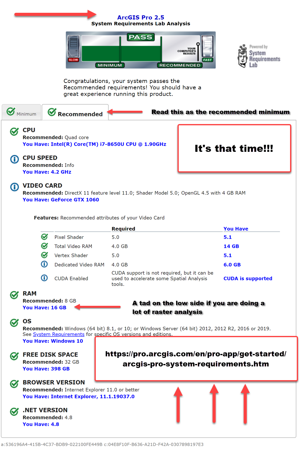
ArcGIS Pro system requirements—ArcGIS Pro | ArcGIS Desktop 

Download, install, and authorize—ArcGIS Pro | ArcGIS Desktop 

2  Go back to step 1.

Really, it is good and should be read, especially the part about your computer being able to run the software

3  My Esri, My Organization, Downloads

If it is there, it will look like the following:

4  Installation steps for retentives

Now, don't hit the Run option!  It is tempting, but there is Save and Save As.  Save As will be used.

To prepare for this, you should have done the following (not!, I am guessing)

•  Make a folder to download your software ....
  • C:\users\you\whatever\downloads ... is no good, just because
  • C:\Computer\ArcGISPro_2x is good... simple, obvious and you own it
  • Download the *.exe to that folder using Save As
• Right-click on the *.exe file and run it as administrator, specifying the above folder as the destination
• Do the same for the *.msi file and you will automagically get a bunch of stuff in that folder AFTER the installation is complete... just follow that, but your folder should look like the following

Where step 1 is the main installation folder you created and downloaded the *.exe (2), when you run the *.exe, you will get the folder in step 3, and run the *.msi and you get the rest of the stuff.

Why do I do this? 

Because if things go really really bad, you will know where the ArcGISPro.msi file is, so when you have to do a complete uninstall, you can reinstall within a minute. 

Simple... no remembering or letting Microsoft Parent decide where things should go

What I did next

I do the conda thing... some legacy but relevant reading

/blogs/dan_patterson/2017/07/01/arcgis-pro-2-creating-desktop-shortcuts 

/blogs/dan_patterson/2018/12/13/spyder 

/blogs/dan_patterson/2018/07/01/arcgis-pro-your-conda-environments 

Crank up conda through whatever means to run ...proenv.bat which sets everything up.  What is show below is what happens when I created a shortcut (Dolly) and messed around with the python ide so it isn't as dark and gloomy as yours will be.

I needed the following to do the programming I need and I did it in the following order.

1  Update numpy

• (arcgispro-py3) C:\arc_pro\bin\Python\envs\arcgispro-py3> conda update numpy

2 Downgrade sphinx to 1.8.5  (needed IF you document your scripts, otherwise the documentation will look horrible)

• (arcgispro-py3) C:\arc_pro\bin\Python\envs\arcgispro-py3> conda install sphinx==1.8.5

3  installed sphinx_rtd_theme   Getting Started with Sphinx — Read the Docs 3.5.3 documentation 

    You can skip this step if you don't do documentation or produce reports, or use Markdown or reStructured Text (or know what I am talking about )

• (arcgispro-py3) C:\arc_pro\bin\Python\envs\arcgispro-py3>conda install sphinx_rtd_theme --no-pin

4  Install spyder

• (arcgispro-py3) C:\arc_pro\bin\Python\envs\arcgispro-py3>conda install spyder

Tips

Never, never install without doing a test run first!

      (arcgispro-py3) ….snip …. >conda install some_package --dry-run 

Then examine what it is going to do.  Sometimes, nothing 'bad' will happen, but you should at least make a copy what you are about to install.  If things go bad, you can roll back through the 'revisions' to a previous state.

Revision History from this install

(arcgispro-py3) C:\arc_pro\bin\Python\envs\arcgispro-py3>conda list --revisions
2019-06-27 20:36:30  (rev 0)  Fresh install of ArcGIS Pro 2.4 in this example
    +arcgis-1.6.1 (esri)
    +arcgispro-2.4 (esri)
    ... huge snip ....
    +zeromq-4.3.1
    +zlib-1.2.11

Now if anything goes wrong, (Assuming I want to go back to revision 1)

A little conda in spyder anyone?

Just remember to change directory into your conda environment (ie cd c:\arc_pro\bin\Python\envs\arcgispro-py3 in my example.

Summary of magic functions (from %lsmagic):

Available line magics:
  %aimport  %alias  %alias_magic  %autoawait  %autocall  %automagic  %autoreload
  %autosave  %bookmark  %cd  %clear  %cls  %colors  %conda  %config  %connect_info
  %copy  %ddir  %debug  %dhist  %dirs  %doctest_mode  %echo  %ed  %edit  %env  %gui
  %hist  %history  %killbgscripts  %ldir  %less  %load  %load_ext  %loadpy  %logoff
  %logon  %logstart  %logstate  %logstop  %ls  %lsmagic  %macro  %magic  %matplotlib
  %mkdir  %more  %notebook  %page  %pastebin  %pdb  %pdef  %pdoc  %pfile  %pinfo
  %pinfo2  %pip  %popd  %pprint  %precision  %prun  %psearch  %psource  %pushd
  %pwd  %pycat  %pylab  %qtconsole  %quickref  %recall  %rehashx  %reload_ext  %ren
  %rep  %rerun  %reset  %reset_selective  %rmdir  %run  %save  %sc  %set_env  %store
  %sx  %system  %tb  %time  %timeit  %unalias  %unload_ext  %varexp  %who  %who_ls
  %whos  %xdel  %xmode

Available cell magics:

  %%!  %%HTML  %%SVG  %%bash  %%capture  %%cmd  %%debug  %%file  %%html  %%javascript
  %%js  %%latex  %%markdown  %%perl  %%prun  %%pypy  %%python  %%python2  %%python3
  %%ruby  %%script  %%sh  %%svg  %%sx  %%system  %%time  %%timeit  %%writefile‍‍‍‍‍‍‍‍‍‍‍‍‍‍‍‍‍‍‍‍‍‍‍‍‍‍‍‍‍‍‍‍‍‍‍‍‍‍‍‍‍‍‍‍‍‍‍‍‍‍‍‍‍‍‍‍‍‍‍‍