- Subscribe to RSS Feed
- Mark as New
- Mark as Read
- Bookmark
- Subscribe
- Printer Friendly Page
Matplotlib
In the ArcGIS ecosystem, I often use Matplotlib to plot geometry objects, particularly when I have a need to save a plot as an image for documentation purposes.
The following code example shows how to plot polygons or polylines relatively quickly. The required inputs are a numpy array or a Geo array.
----
The plots to the left show variants of polygon geometry displayed as polylines or filled polygons. The plot to the right is for a hexagon geometry. The geometry values as arrays are shown below their respective plots. Geometries with holes and/or different point compositions are represented as object arrays (aka 'ragged arrays'), while regular patterns are simple numpy ndarrays. Compose your own for testing or extract list values from json data.
array([array([[ 0.0, 0.0], [ 0.0, 10.0], [ 8.0, 10.0], [ 10.0, 10.0],
[ 10.0, 8.0], [ 10.0, 0.0], [ 0.0, 0.0]]),
array([[ 3.0, 3.0], [ 7.0, 3.0], [ 5.0, 7.0], [ 3.0, 3.0]]),
array([[ 8.0, 10.0], [ 8.0, 11.0], [ 8.0, 12.0], [ 12.0, 12.0],
[ 12.0, 8.0], [ 10.0, 8.0], [ 10.0, 10.0], [ 8.0, 10.0]]),
array([[ 5.0, 11.0], [ 5.0, 12.0], [ 6.0, 12.0], [ 8.0, 12.0],
[ 8.0, 11.0], [ 5.0, 11.0]]),
array([[ 5.0, 12.0], [ 5.0, 15.0], [ 6.0, 15.0], [ 6.0, 12.0],
[ 5.0, 12.0]])], dtype=object)
array([[[-1.0, 0.0], [-0.5, 0.9], [ 0.5, 0.9], [ 1.0, 0.0], [ 0.5, -0.9],
[-0.5, -0.9], [-1.0, -0.0]], [[ 0.5, 0.9], [ 1.0, 1.7],
[ 2.0, 1.7], [ 2.5, 0.9], [ 2.0, 0.0], [ 1.0, -0.0], [ 0.5, 0.9]],
... snip ...
[[ 3.5, 4.3], [ 4.0, 5.2], [ 5.0, 5.2], [ 5.5, 4.3], [ 5.0, 3.5],
[ 4.0, 3.5], [ 3.5, 4.3]], [[ 5.0, 3.5], [ 5.5, 4.3], [ 6.5, 4.3],
[ 7.0, 3.5], [ 6.5, 2.6], [ 5.5, 2.6], [ 5.0, 3.5]]]) 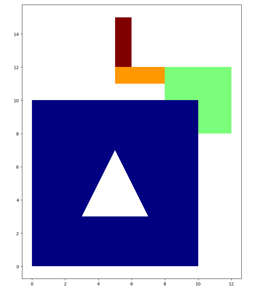 | 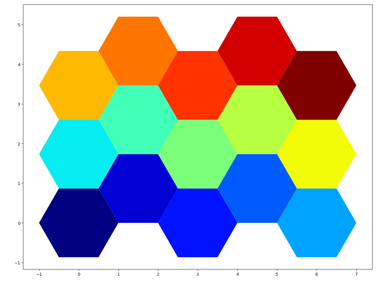 |
The code is below. NumPy documentation style is used for the __doc__ string.
import numpy as np
import matplotlib.pyplot as plt
from matplotlib.collections import LineCollection
def plot_polygons(arr, outline=True):
"""Plot Geo array poly boundaries.
Parameters
----------
arr : ndarray or Geo array
If the arrays is a Geo array, it will convert it to `arr.bits`.
outline : boolean
True, returns the outline of the polygon. False, fills the polygon
References
----------
See module docs for general references.
Example
-------
use hexs to demonstrate::
h = npg.npg_create.hex_flat(dx=1, dy=1, x_cols=5, y_rows=3,
orig_x=0, orig_y=0, kind=2, asGeo=True)
"""
def _line(p, plt): # , arrow=True): # , color, marker, linewdth):
"""Connect the points."""
X, Y = p[:, 0], p[:, 1]
plt.plot(X, Y, color='black', linestyle='solid', linewidth=2)
# ----
if hasattr(arr, 'IFT'):
cw = arr.CW
shapes = arr.bits
else:
cw = np.repeat(1, arr.shape[0])
shapes = np.copy(arr)
fig, ax = plt.subplots(1, 1)
fig.set_figheight = 8
fig.set_figwidth = 8
fig.dpi = 200
plt.tight_layout(pad=0.2, h_pad=0.1, w_pad=0.1)
ax.set_aspect('equal', adjustable='box')
# cmap = plt.cm.get_cmap(plt.cm.viridis, 143) # default colormap
cmap = plt.cm.get_cmap('jet', len(shapes)) # 'hsv'
for i, shape in enumerate(shapes):
if outline: # _line(shape, plt) # alternate, see line for options
plt.fill(*zip(*shape), facecolor='none', edgecolor='black',
linewidth=3)
else:
if cw[i] == 0:
clr = "w"
else:
clr = cmap(i) # clr=np.random.random(3,) # clr = "b"
plt.fill(*zip(*shape), facecolor=clr)
# ----
plt.show()
return plt
# ---------------------------------------------------------------------
if __name__ == "__main__":
"""Main section... """
"""
# --- sample hexagons
z = np.array([[[-1.0, 0.0],
[-0.5, 0.9],
[ 0.5, 0.9],
[ 1.0, 0.0],
[ 0.5, -0.9],
[-0.5, -0.9],
[-1.0, -0.0]],
[[ 0.5, 0.9],
[ 1.0, 1.7],
[ 2.0, 1.7],
[ 2.5, 0.9],
[ 2.0, 0.0],
[ 1.0, -0.0],
[ 0.5, 0.9]],
[[ 2.0, 0.0],
[ 2.5, 0.9],
[ 3.5, 0.9],
[ 4.0, 0.0],
[ 3.5, -0.9],
[ 2.5, -0.9],
[ 2.0, -0.0]]])
plot_polygons(z, outline=False) # ---- plot filled
"""
A couple of sample hexagons are given in lines 65-87 and the function call on line 89, if you want to experiment.
If you are interested in geometry, then I have been working on this as part of my Free Tools project. The main/most current code is contained in this link.
Have fun.
You must be a registered user to add a comment. If you've already registered, sign in. Otherwise, register and sign in.