Turn on suggestions
Auto-suggest helps you quickly narrow down your search results by suggesting possible matches as you type.
Cancel
- Home
- :
- All Communities
- :
- Services
- :
- Esri Training
- :
- Esri Training Matters Blog
- :
- GIS Analysis: Planning to Prepare Your Data Pays O...
GIS Analysis: Planning to Prepare Your Data Pays Off
Subscribe
4255
0
01-26-2012 01:28 PM
- Subscribe to RSS Feed
- Mark as New
- Mark as Read
- Bookmark
- Subscribe
- Printer Friendly Page
01-26-2012
01:28 PM
"If you fail to plan, you plan to fail." This old adage has wide applicability—when you want to lose 10 pounds, be picked for a leadership position, land the perfect job, and on and on. So just like everything else in life, when it comes to GIS analysis, planning pays off. To ensure reliable results, here's the tried and true process we recommend:
Step 2 is arguably the most critical as your final results are only as reliable as the data you start with. Read on for a closer look at exploring and preparing data for an analysis project.Exploring Data
The first part of step 2 flows directly from the analysis question. Spend time upfront identifying all the data, including attributes, needed to answer the question. Don't get halfway through a project and discover you're missing a key dataset.
The point of exploring data is to understand what valid things you can do with it. You should:
Preparing data means ensuring datasets can be validly analyzed together and reducing processing time as much as possible. Data preparation tasks often include projecting data, reducing the spatial extent to the area of interest, deleting unneeded attributes, creating new attributes, cleaning up attribute values, and more.
Get the most out of ArcGIS geoprocessing tools. Many can be run in batch mode and some have options you can use to combine data preparation tasks. For example, inside the Feature Class to Feature Class tool, you can create a SQL expression to import only features located in your area of interest, you can exclude source attributes you don't need, and you can define new attribute fields that you do need. With one tool, you accomplish three preparation steps.
You can also create a model to automate data preparation—just drag the geoprocessing tools you need into a model window and define their parameters. Creating a model is an excellent way to visualize and order tasks as you go.
The same data may be used for multiple analyses. It's good practice to make a copy of the original data before you make changes to prepare for a specific project. This way, the original data is preserved for subsequent analyses—and you have something to go back to just in case.Example: Analyze Piracy Incidents
Let's look at a simple example to illustrate the importance of exploring and preparing data. The analysis question has been framed as:
The U.S. National Geospatial-Intelligence Agency (NGA) distributes Anti-Shipping Activity Messages (ASAM) reports, which include locations and descriptions of hostile acts against ships and mariners worldwide. You can download ASAM data in shapefile format from the NGA website.Explore the Data
After downloading the ASAM shapefile, add it to ArcMap. For geographic context, it helps to add a basemap; in this case, the World Topograpic Map from ArcGIS Online works well.
The map graphic on the right shows the global extent of the ASAM data (symbolized with red dots). A quick exploration of the attribute table reveals 6,158 records; an attribute that stores a world subregion code; and an attribute that stores the date each incident occurred—the date range is 5/1/1978 through 1/9/2012.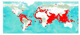
To efficiently answer the analysis question, you need to reduce the data to incidents that occurred between 1/1/2009 and 12/31/2011 in subregion 62 (the NGA website lists subregion codes). You also need to do some other preparation work to resolve issues with this data.Issue 1: The data has no spatial reference.
When the ASAM shapefile was added to ArcMap, a message that the data was missing a spatial reference displayed. For shapefiles, spatial reference information is stored in the projection (.PRJ) file and it's not unusual for the .PRJ file to be missing, as it is here. So how do you know which coordinate system to use?
A good place to start is the Layer Properties dialog box. In the Source tab, when you look at the extent coordinates, the number of digits to the left of the decimals tells you it's a geographic coordinate system.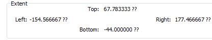
Since the data has a global extent, it is reasonable to assign the WGS 1984 geographic coordinate system. If your analysis involved precise measurements, you would want to assign a suitable projected coordinate system for the area of interest as well.Issue 2: The data is more extensive than you need.
The ASAM data has a larger spatial extent and a longer temporal extent than you need. SQL queries will resolve these issues.
For this analysis, the initial data preparation tasks are:
1. Create a file geodatabase to organize the project data.
2. Import the ASAM shapefile into the file geodatabase.
3. Assign the WGS 1984 coordinate system to the geodatabase feature class.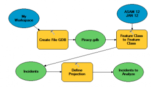
The model graphic on the right shows the geoprocessing workflow.
A SQL expression was defined in the Feature Class to Feature Class tool dialog so only the incidents meeting the analysis criteria will be imported.
After running the model, you have a new feature class with 643 features. Now that the data is a more manageable size, before moving on to step 3 of the analysis process, you need to verify that all 643 features represent piracy incidents that occurred during the analysis timeframe.
In ASAM data, two fields contain date information (Reference and DateOfOcc). DateOfOcc stores mm/dd/yyyy, while Reference includes the year followed by a unique ID number. The Reference field was used in the Feature Class to Feature Class dialog's SQL expression for convenience, but it means there's cleanup to be done now. Sorting the DateOfOcc field reveals that four records have 2009 in the Reference field (reflecting the year the report was submitted), but their DateOfOcc values tell you the incidents actually occurred during the last week of 2008. These records can be deleted. Now there are 639 records to analyze.Issue 3: Attribute values are inconsistent.
Next, you need to make sure all records are incidents of piracy. The Aggressor field stores this information. Sorting the Aggressor field reveals multiple values, the vast majority of which contain some variation of "pirate."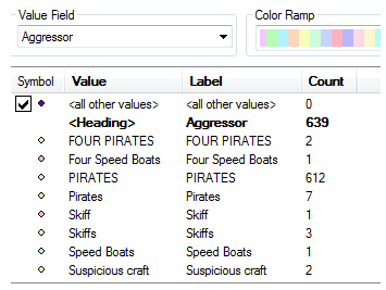
After exploring the Aggressor values, you can create an attribute query to select all records that have one of the "pirate" variations in the Aggressor field, then switch the selection to see how many records don't directly reference pirate aggressors. In this case, only 16 incidents have Aggressor values that don't reference pirates.
You need to explore the incident descriptions to determine whether any of these 16 likely were attacks by pirates. If they clearly did not involve pirate aggressors, delete the records. In this case, the incident descriptions don't clearly rule out pirate aggressors, so you choose to keep the records but categorize them to account for the ambiguity. You use the Field Calculator to change those 16 Aggressor values to Possible Pirates, and you clean up the remaining records so they all have an Aggressor value of Pirates.Issue 4: The table has duplicate records.
With the DateOfOcc field sorted, a look at the Reference field shows something alarming. There seem to be many duplicate records—records with the same Reference value and identical data in the other attribute fields. How could this be? Did something go wrong when you converted the shapefile to a geodatabase feature class?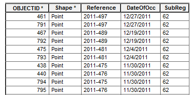
This is the time to go back to the original data and determine if the duplicates existed there. Because of the number of features in the shapefile, it's efficient to summarize the Reference field, which outputs a table with a count of each unique reference value in the shapefile.
After creating the summary table and sorting the Count_Reference field, you see that many Reference numbers have a duplicate. To find out exactly how many, select the records whose Count_Reference value is equal to 2. It turns out that 493 Reference numbers have a duplicate in the source data you started with. Determining how many of those 493 are in your geodatabase feature class requires more work.
Just like you did for the shapefile, in the Incidents to Analyze layer, summarize the Reference field to output a table with a count of reference values, then select the records whose Count_Reference value is equal to 2. It turns out that 170 records have a duplicate. Is there a way to easily remove 170 duplicate records? Yes, fairly easily. Here's how:
Final result: 469 incidents ready to be used as input in step 3 of the GIS analysis process.
All this data exploring and preparing really only required a couple of hours of focused work. Of course, the incident victim values likely need cleanup as well—but we'll end the example here as the boundary line between steps 2 and 3 of the GIS analysis process is not a solid fence.Takeaway: When preparing data for analysis, you have to make decisions and live with some uncertainty. Your specific analysis criteria and how well you know the topic determine how far you go to clean up the data. To avoid creating or propagating errors, carefully explore the data and document any data preparation you do and why you chose to do it. Remember that a model is a valuable tool to document your workflow and help others better understand your analysis results.
The data you use for a GIS analysis project may not be perfect and it may not fit your needs exactly. But planning and preparation go a long way toward making sure the data generates reliable results you can confidently share with others.
Want to learn more best practices for GIS analysis? Here are courses that can help.
- Frame the question.
- Explore and prepare data.
- Choose analysis methods and tools.
- Perform the analysis.
- Examine and refine results.
Step 2 is arguably the most critical as your final results are only as reliable as the data you start with. Read on for a closer look at exploring and preparing data for an analysis project.Exploring Data
The first part of step 2 flows directly from the analysis question. Spend time upfront identifying all the data, including attributes, needed to answer the question. Don't get halfway through a project and discover you're missing a key dataset.
The point of exploring data is to understand what valid things you can do with it. You should:
- Examine the metadata. Note the spatial resolution and accuracy, coordinate system, when the data was collected and by whom, data use constraints, and other important information.
- Explore all the spatial datasets you plan to use in ArcMap. Do the layers align properly together? Are some layers more generalized than others? Do some layers have a larger (or smaller) extent than needed?
- Explore the attribute table for each layer and note the number of records and the attributes. Sort fields and look at field statistics to understand the values. Note obvious data entry errors and inconsistencies.
Preparing data means ensuring datasets can be validly analyzed together and reducing processing time as much as possible. Data preparation tasks often include projecting data, reducing the spatial extent to the area of interest, deleting unneeded attributes, creating new attributes, cleaning up attribute values, and more.
Get the most out of ArcGIS geoprocessing tools. Many can be run in batch mode and some have options you can use to combine data preparation tasks. For example, inside the Feature Class to Feature Class tool, you can create a SQL expression to import only features located in your area of interest, you can exclude source attributes you don't need, and you can define new attribute fields that you do need. With one tool, you accomplish three preparation steps.
You can also create a model to automate data preparation—just drag the geoprocessing tools you need into a model window and define their parameters. Creating a model is an excellent way to visualize and order tasks as you go.
The same data may be used for multiple analyses. It's good practice to make a copy of the original data before you make changes to prepare for a specific project. This way, the original data is preserved for subsequent analyses—and you have something to go back to just in case.Example: Analyze Piracy Incidents
Let's look at a simple example to illustrate the importance of exploring and preparing data. The analysis question has been framed as:
- In the years 2009 through 2011, what types of vessels were the most frequent victims of piracy in and around the Gulf of Aden and Arabian Sea?
The U.S. National Geospatial-Intelligence Agency (NGA) distributes Anti-Shipping Activity Messages (ASAM) reports, which include locations and descriptions of hostile acts against ships and mariners worldwide. You can download ASAM data in shapefile format from the NGA website.Explore the Data
After downloading the ASAM shapefile, add it to ArcMap. For geographic context, it helps to add a basemap; in this case, the World Topograpic Map from ArcGIS Online works well.
The map graphic on the right shows the global extent of the ASAM data (symbolized with red dots). A quick exploration of the attribute table reveals 6,158 records; an attribute that stores a world subregion code; and an attribute that stores the date each incident occurred—the date range is 5/1/1978 through 1/9/2012.
To efficiently answer the analysis question, you need to reduce the data to incidents that occurred between 1/1/2009 and 12/31/2011 in subregion 62 (the NGA website lists subregion codes). You also need to do some other preparation work to resolve issues with this data.Issue 1: The data has no spatial reference.
When the ASAM shapefile was added to ArcMap, a message that the data was missing a spatial reference displayed. For shapefiles, spatial reference information is stored in the projection (.PRJ) file and it's not unusual for the .PRJ file to be missing, as it is here. So how do you know which coordinate system to use?
A good place to start is the Layer Properties dialog box. In the Source tab, when you look at the extent coordinates, the number of digits to the left of the decimals tells you it's a geographic coordinate system.
- With geographic coordinate systems, the Left and Right extent values will have one to three digits to the left of the decimal, while the Top and Bottom extent values will have one or two digits to the left of the decimal.
- Tip: You can learn methods to identify unknown coordinate systems in the Working with Coordinate Systems in ArcGIS web course.
Since the data has a global extent, it is reasonable to assign the WGS 1984 geographic coordinate system. If your analysis involved precise measurements, you would want to assign a suitable projected coordinate system for the area of interest as well.Issue 2: The data is more extensive than you need.
The ASAM data has a larger spatial extent and a longer temporal extent than you need. SQL queries will resolve these issues.
For this analysis, the initial data preparation tasks are:
1. Create a file geodatabase to organize the project data.
2. Import the ASAM shapefile into the file geodatabase.
- Import only features within subregion 62 that fall within the date range 1/1/2009-12/31/2011.
3. Assign the WGS 1984 coordinate system to the geodatabase feature class.

The model graphic on the right shows the geoprocessing workflow.
A SQL expression was defined in the Feature Class to Feature Class tool dialog so only the incidents meeting the analysis criteria will be imported.
- Tip: If you need help creating a SQL expression, use the SQL reference in the ArcGIS Help.
After running the model, you have a new feature class with 643 features. Now that the data is a more manageable size, before moving on to step 3 of the analysis process, you need to verify that all 643 features represent piracy incidents that occurred during the analysis timeframe.
In ASAM data, two fields contain date information (Reference and DateOfOcc). DateOfOcc stores mm/dd/yyyy, while Reference includes the year followed by a unique ID number. The Reference field was used in the Feature Class to Feature Class dialog's SQL expression for convenience, but it means there's cleanup to be done now. Sorting the DateOfOcc field reveals that four records have 2009 in the Reference field (reflecting the year the report was submitted), but their DateOfOcc values tell you the incidents actually occurred during the last week of 2008. These records can be deleted. Now there are 639 records to analyze.Issue 3: Attribute values are inconsistent.
Next, you need to make sure all records are incidents of piracy. The Aggressor field stores this information. Sorting the Aggressor field reveals multiple values, the vast majority of which contain some variation of "pirate."

- Tip: A quick visual method to understand how the Aggressor values vary is to open the Layer Properties dialog box and symbolize the layer by Unique Values based on the Aggressor field. Each unique aggressor value displays and the Count field tells you how many of each.
After exploring the Aggressor values, you can create an attribute query to select all records that have one of the "pirate" variations in the Aggressor field, then switch the selection to see how many records don't directly reference pirate aggressors. In this case, only 16 incidents have Aggressor values that don't reference pirates.
You need to explore the incident descriptions to determine whether any of these 16 likely were attacks by pirates. If they clearly did not involve pirate aggressors, delete the records. In this case, the incident descriptions don't clearly rule out pirate aggressors, so you choose to keep the records but categorize them to account for the ambiguity. You use the Field Calculator to change those 16 Aggressor values to Possible Pirates, and you clean up the remaining records so they all have an Aggressor value of Pirates.Issue 4: The table has duplicate records.
With the DateOfOcc field sorted, a look at the Reference field shows something alarming. There seem to be many duplicate records—records with the same Reference value and identical data in the other attribute fields. How could this be? Did something go wrong when you converted the shapefile to a geodatabase feature class?
This is the time to go back to the original data and determine if the duplicates existed there. Because of the number of features in the shapefile, it's efficient to summarize the Reference field, which outputs a table with a count of each unique reference value in the shapefile.
After creating the summary table and sorting the Count_Reference field, you see that many Reference numbers have a duplicate. To find out exactly how many, select the records whose Count_Reference value is equal to 2. It turns out that 493 Reference numbers have a duplicate in the source data you started with. Determining how many of those 493 are in your geodatabase feature class requires more work.
Just like you did for the shapefile, in the Incidents to Analyze layer, summarize the Reference field to output a table with a count of reference values, then select the records whose Count_Reference value is equal to 2. It turns out that 170 records have a duplicate. Is there a way to easily remove 170 duplicate records? Yes, fairly easily. Here's how:
- Join the summary table of reference values to the Incidents to Analyze table.
- Select records whose Count_Reference value is equal to 2—as expected, there are 340 selected records.
- Start an edit session, then use the Delete Identical tool to delete the selected records that have the same Reference value as another record (note that before running the Delete Identical tool, you must remove the table join—the selected records remain selected after the join is removed).
Final result: 469 incidents ready to be used as input in step 3 of the GIS analysis process.
All this data exploring and preparing really only required a couple of hours of focused work. Of course, the incident victim values likely need cleanup as well—but we'll end the example here as the boundary line between steps 2 and 3 of the GIS analysis process is not a solid fence.Takeaway: When preparing data for analysis, you have to make decisions and live with some uncertainty. Your specific analysis criteria and how well you know the topic determine how far you go to clean up the data. To avoid creating or propagating errors, carefully explore the data and document any data preparation you do and why you chose to do it. Remember that a model is a valuable tool to document your workflow and help others better understand your analysis results.
The data you use for a GIS analysis project may not be perfect and it may not fit your needs exactly. But planning and preparation go a long way toward making sure the data generates reliable results you can confidently share with others.
Want to learn more best practices for GIS analysis? Here are courses that can help.
Labels
You must be a registered user to add a comment. If you've already registered, sign in. Otherwise, register and sign in.
About the Author
Suzanne is a Maryland native who enjoys writing about Esri technology, GIS professional development, and other topics. She is the Training Marketing Manager with Esri Training Services in Redlands, California.
Labels
-
ArcGIS Desktop
26 -
ArcGIS Step by Step
46 -
Class Resources
18 -
e-Learning
62 -
MOOCs
28 -
Software Demos
10 -
Technical Certification
16