ArcGIS Data Interoperability Blog - Page 6

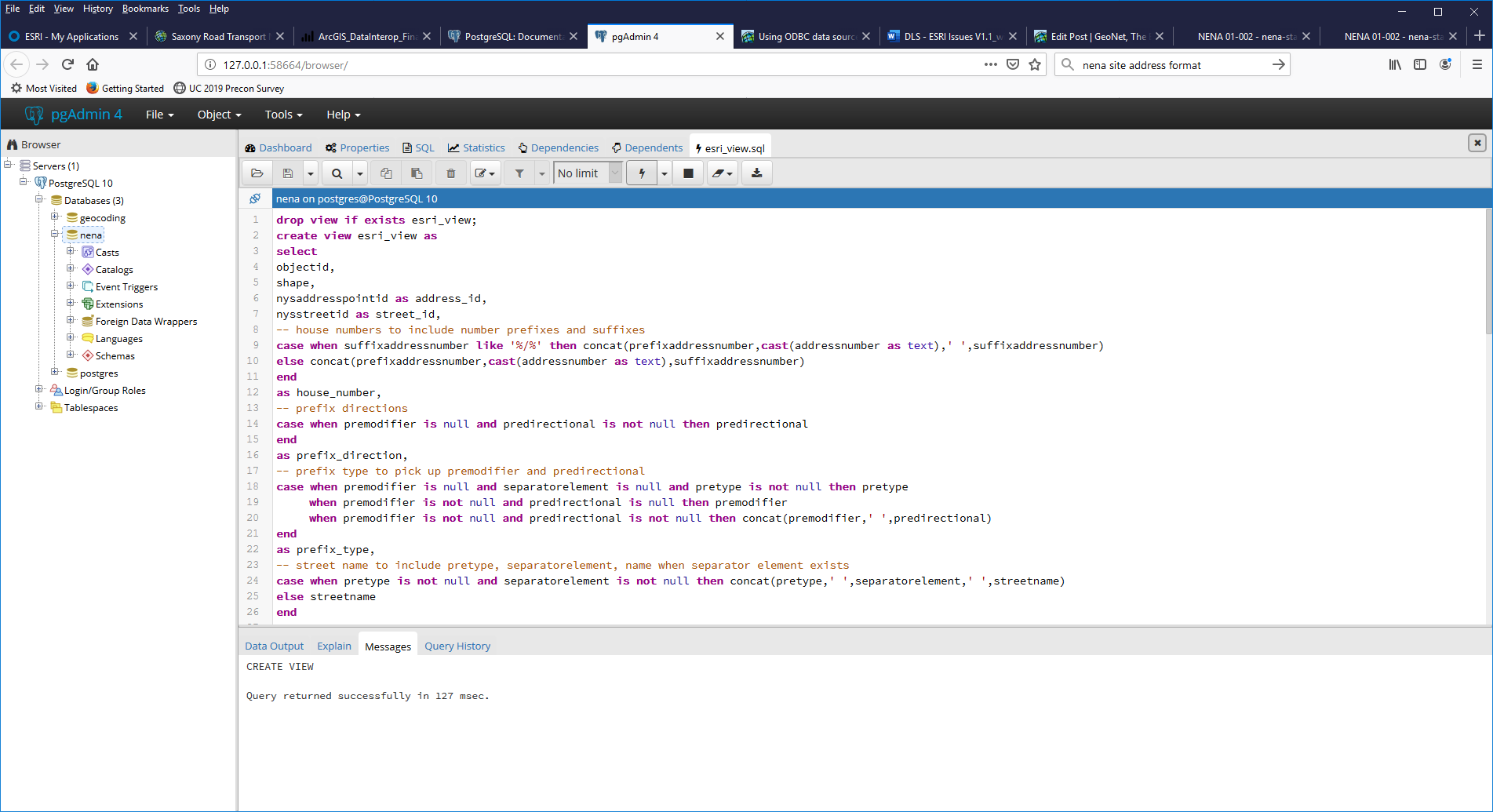
This post shows some advanced ETL techniques but additionally shows how you can hand off finalizing your data to a geodatabase view (actually hundreds of them in this sample), letting the database do the heavy lifting, and in a File GDB at that.  That's right - File Geodatabase views are a new feature at ArcGIS Pro 2.6, due out mid 2020, this is your preview!  No longer are you confined to the 'where' clause in leveraging SQL when working with FileGDB!

I'm going big with the data behind the post - the USDA National Agricultural Statistics Service (NASS) crops database.  I was thinking of calling the post something like 'You, Big Data and Asparagus' but that would lose a lot of people right at the title, even if they do like big data or asparagus.  NASS is a big program, and I don't pretend to know all it offers, but for my demonstration purposes I'll use crop statistics per county.  If you surf the NASS site you'll find ways to access data including selecting areas of interest using a map interface or as compressed text for data focusing on specific topics.  I want it all, in bulk.  NASS supports my need at this FTP site.  The file names change daily, but look for the file beginning 'qs.crops'.  At time of writing it contains over 19 million statistics for over 180 crop types, with records dating from the early 20th century.  So, while the record count might not impress you, I'm going to call NASS 'Big Data' as it has a daily update velocity.

We're going to automate putting this data into File Geodatabase so it can be mapped and analyzed, and doing so at any frequency including the data's native daily lifecycle.

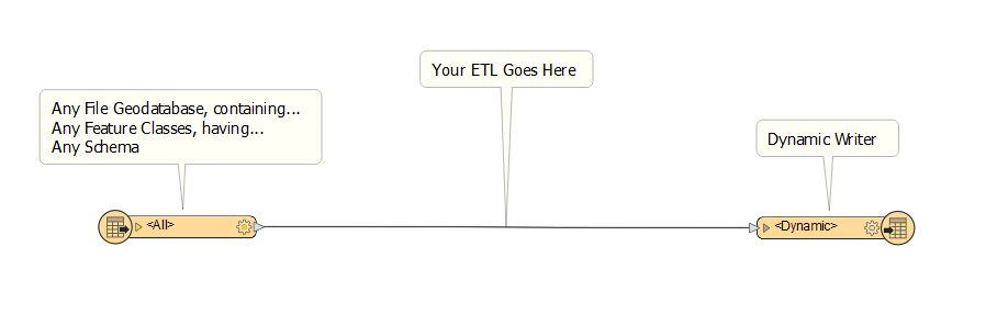
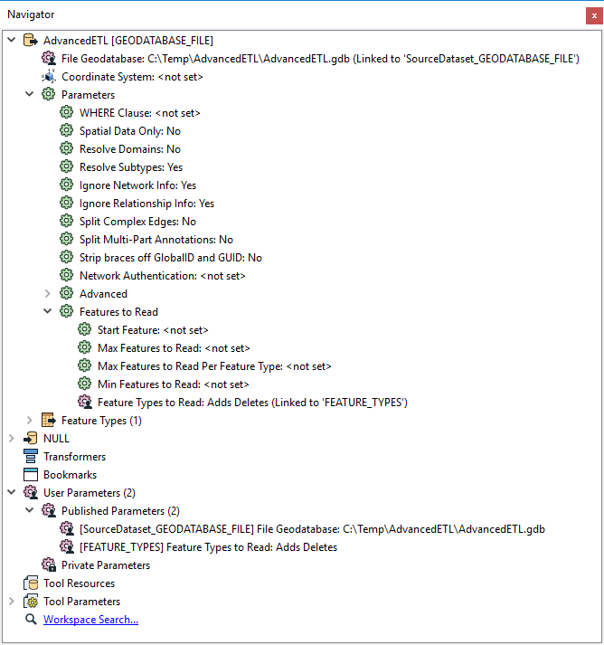
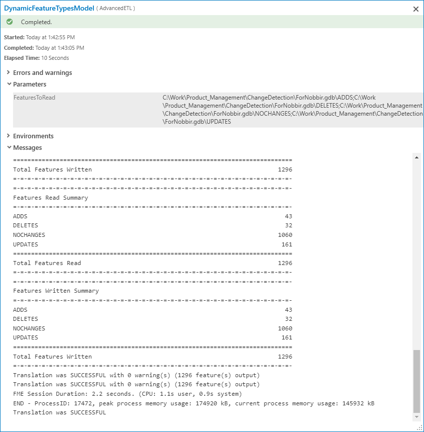
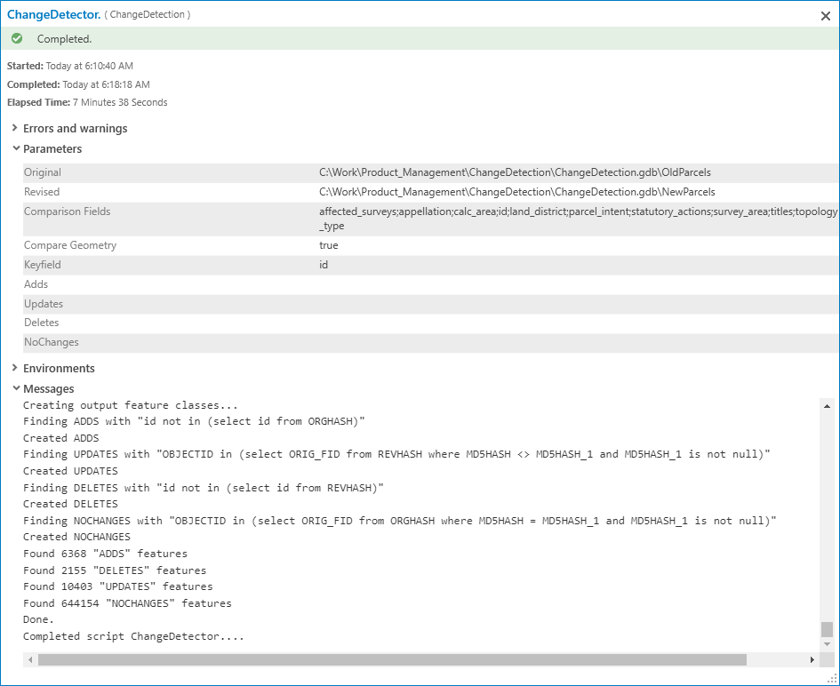
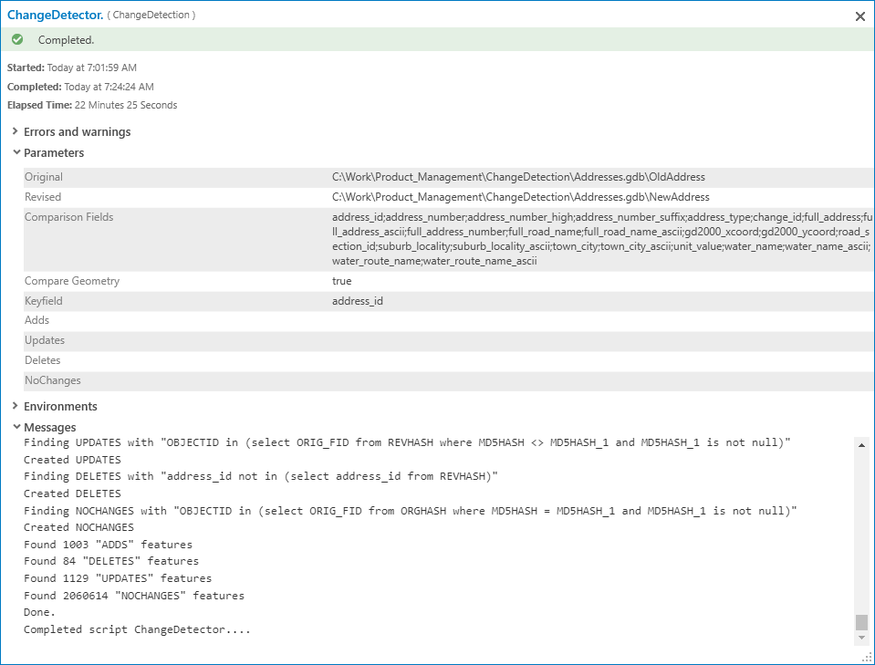
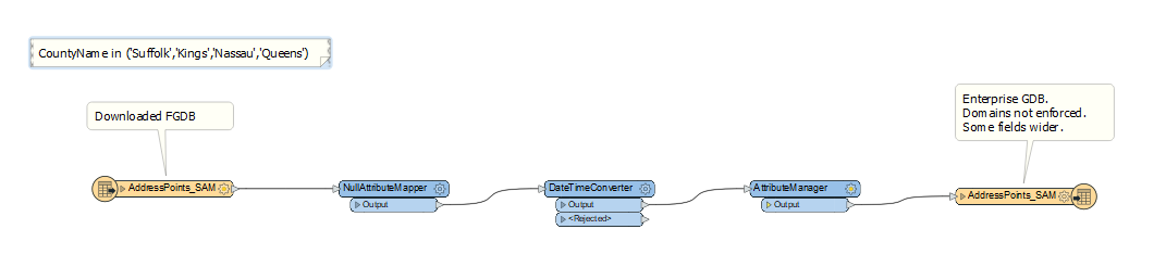
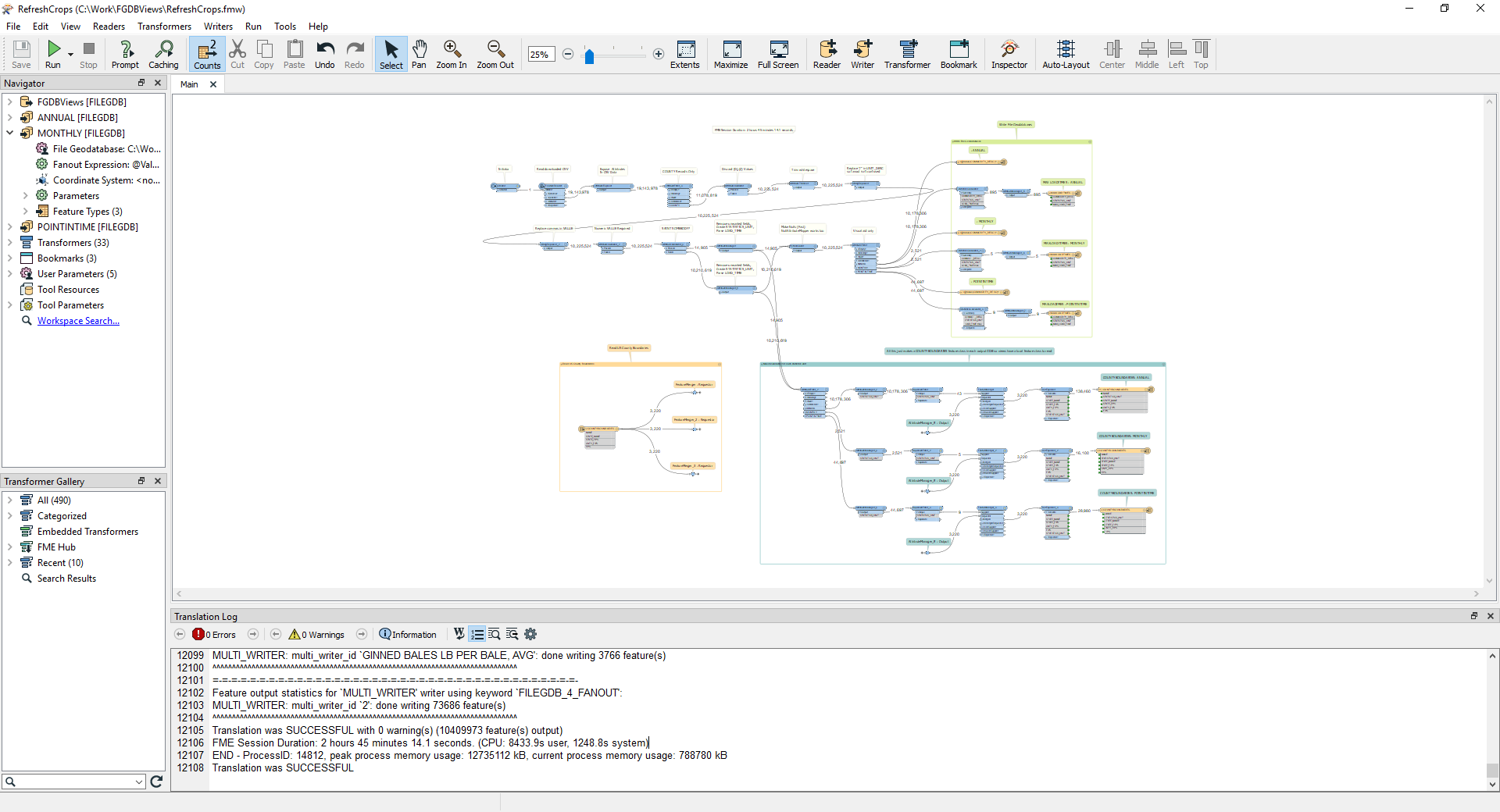
Importing the data to File GDB is done by the ETL tool RefreshCrops (in the post download).  Here is how it looks after a successful run (click to enlarge), we'll walk through the underlying processing next.  (I'm anticipating the reader is able to open the ETL tool, has some Workbench app experience, and will follow along; this requires Data Interoperability extension, or FME, both at release 2020 or later.)

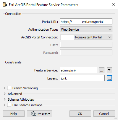
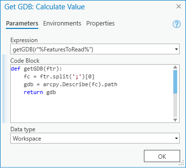
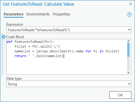
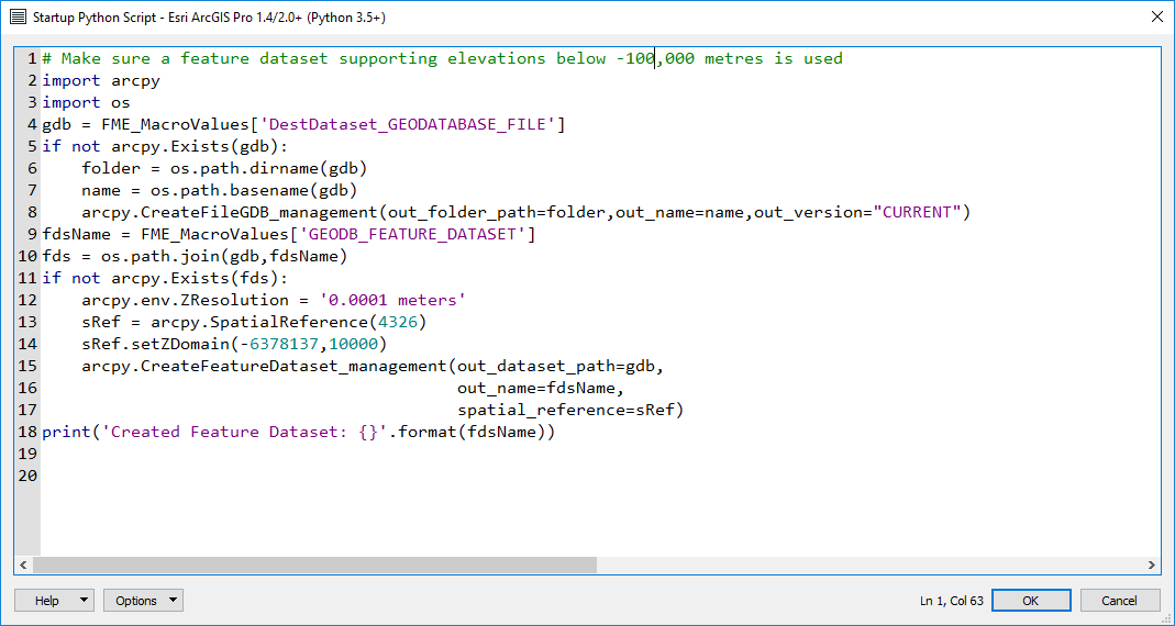
The first issue with the data is that the file of interest changes name daily, so while you could read it with an FTPCaller transformer it would be an error-prone user experience to enter the correct URL for each run, so the process is automated with a Python scripted parameter.  If you have never heard of scripted parameters before, they are a way to make user parameters work dynamically.  We're breaking the no-code paradigm here, but we have a good reason.  Here is how the parameter looks in the property editor:

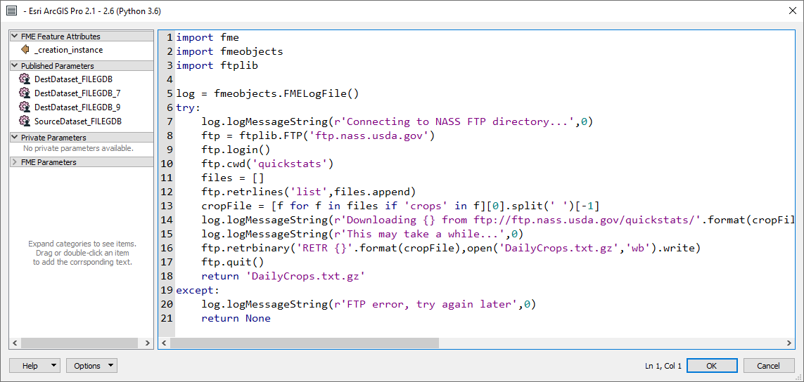
The code opens the FTP site, reads the available file names, then downloads the 'qs.crops' file to a file named DailyCrops.txt.gz.  The file is written into the same folder as the ETL tool, namely the project home folder.  On my laptop it takes a minute or two, and this occurs at the beginning of the tool run.

Now the GZipped payload has to be unpacked.  It is delimited text data so can be opened with a FeatureReader using CSV format.  CSV data rarely travels with a schema.ini file revealing its field types, but the schema is discoverable here, just click the Usage option.  The file is however monolithic, containing all statistics for all crops and multiple aggregation areas (county, state, national) in just the one file, plus three aggregation periods (annual, monthly and point-in-time).  For my purposes I'm interested only in statistics for the County level.  So how do we separate the data by crop and county-level statistic?  The technique is called fanout, in this case two types of fanout are used, dataset fanout that directs records into separate File GDBs for each statistic, and featuretype fanout that directs records into separate tables within each dataset.

The three output parameters (folders for annual, monthly and point in time statistics) have dataset fanout taken from the value of the STATISTICS_UNIT field, which is calculated at run time by concatenating STATISTICCAT_DESC and UNIT_DESC fields.

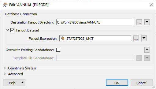
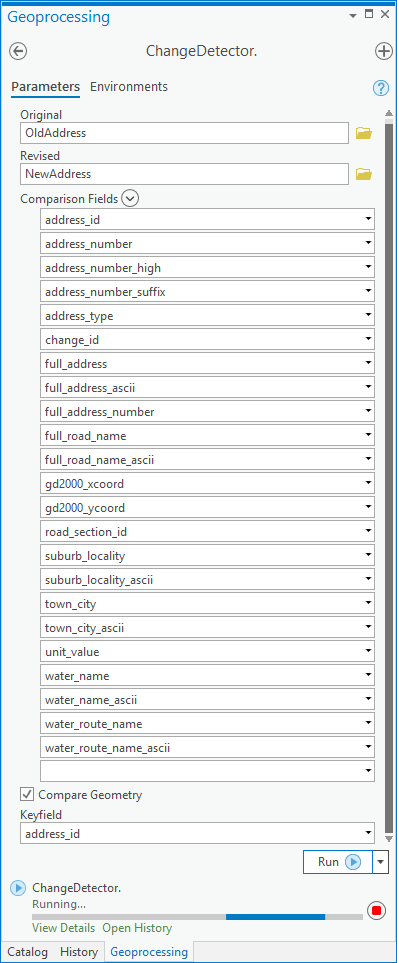
Each output dataset has writers for crop statistics where featuretype fanout is taken from the value of the COMMODITY_DESC field.  Here is the property dialog for ANNUAL statistics:

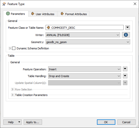
Note also the table handling property is set to Drop and Create, this is so re-runs of the tool remake each crop statistic table and don't keep adding to previously created data.

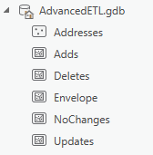
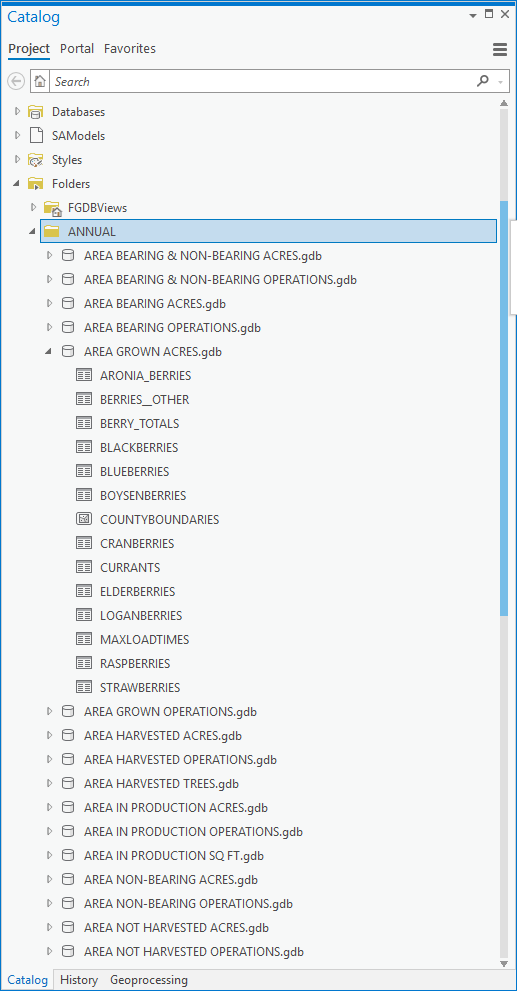
This combination of fanout settings dynamically creates 43 File GDBs for annual statistics, each with as many tables as there are crops reporting the statistic.  There are smaller numbers of monthly and point-in-time workspaces output.  Here is how the ANNUAL folder looks after the initial run (this takes a little less than 3 hours on my laptop):

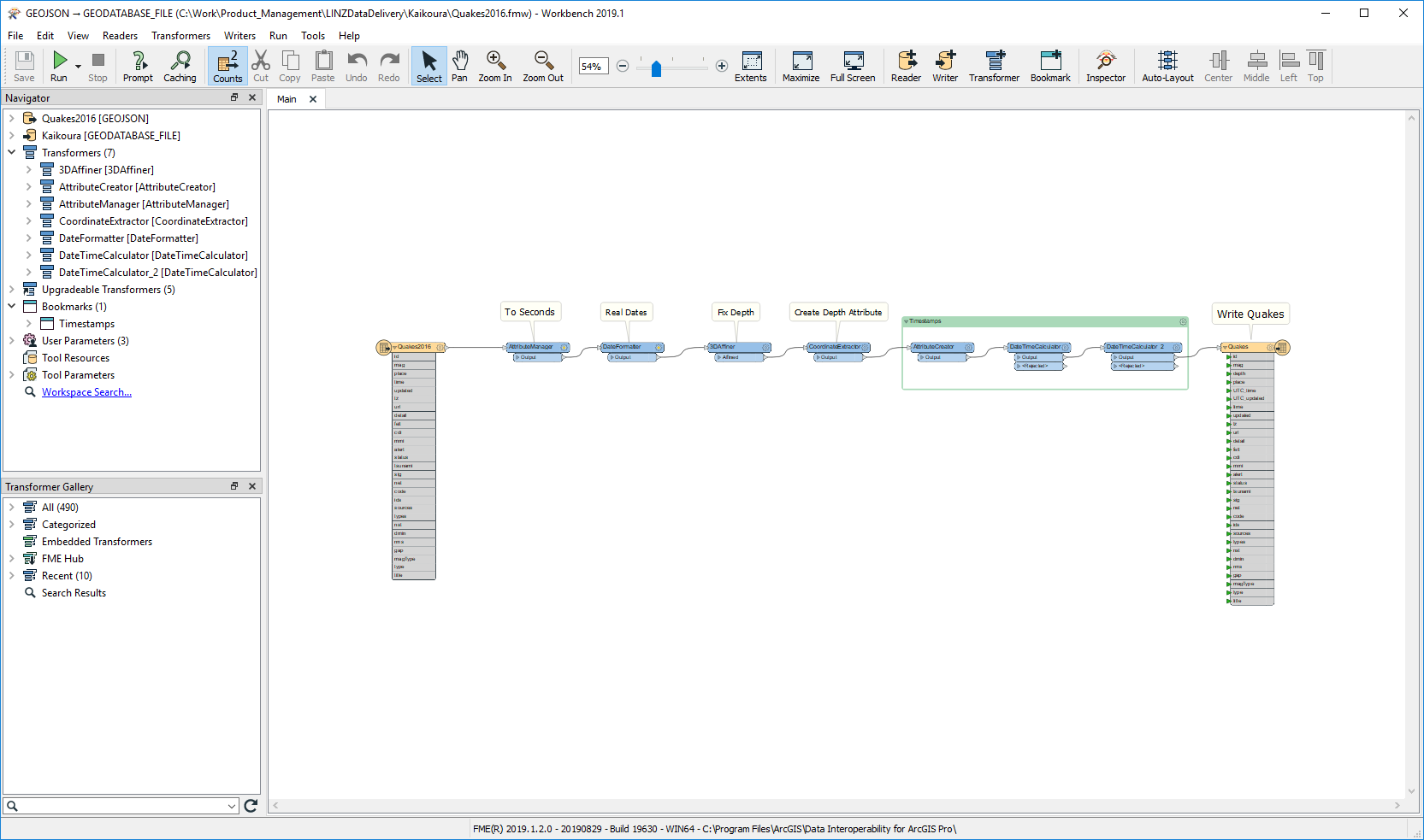
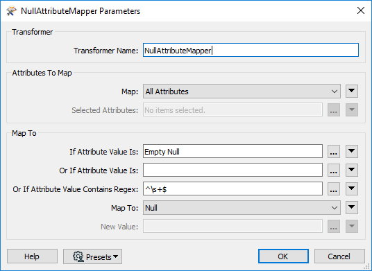
You can inspect the processing in the transformers that are outside of bookmarks and see that the basic idea is to ensure the VALUE field contains a valid numeric value and that the fanout attributes and state & county naming fields are well formed.  The LOAD_TIME field is also made into a correct datetime value.  Otherwise what went in is what comes out into each crop statistic table.  Here is the schema:

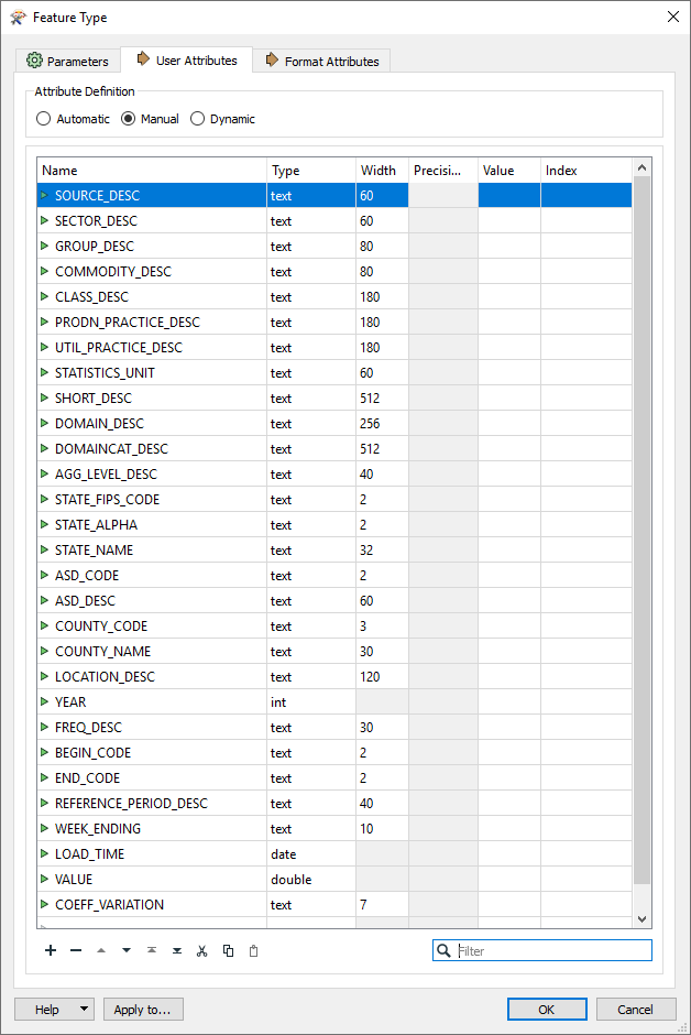
You will notice a feature class COUNTYBOUNDARIES is also copied into each output workspace so that the forthcoming view creation step can use objects within a single File GDB.  A fine point; I use the API-based FILEGDB writer to output COUNTYBOUNDARIES as it has the ability to create an index on county and state name fields; the indexes will be used by the join processor when views are calculated.  These indexes would be created automatically by the underlying Create Database View geoprocessing tool but I like to roll up these background tasks into my ETL.

Another output for each dataset is a table MAXLOADTIMES that shows the time of the latest load time for each crop statistic.  More on this later.

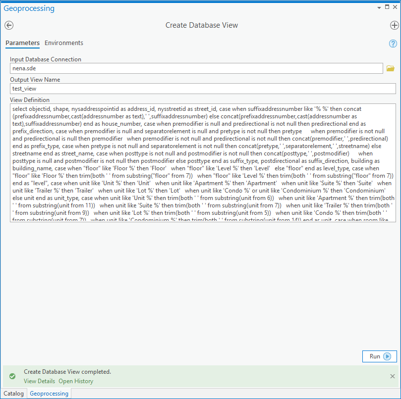
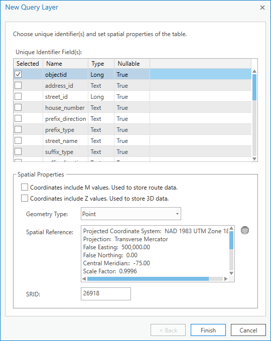
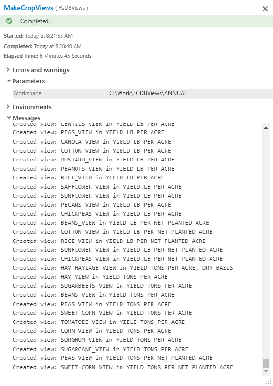
At this point we are ready for view creation.  The input CSV data has no geometry, the whole point of the views is to join county boundary geometry to each crop statistic table.  The script tool MakeCropViews walks each output dataset and creates views from all the crop statistic tables, using the Create Database View tool.  For the ANNUAL folder this makes 895 views in a little over 15 minutes.  Now that is a lot of data you don't have to generate manually!

Here is what you'll see in the message stream as MakeCropViews runs:

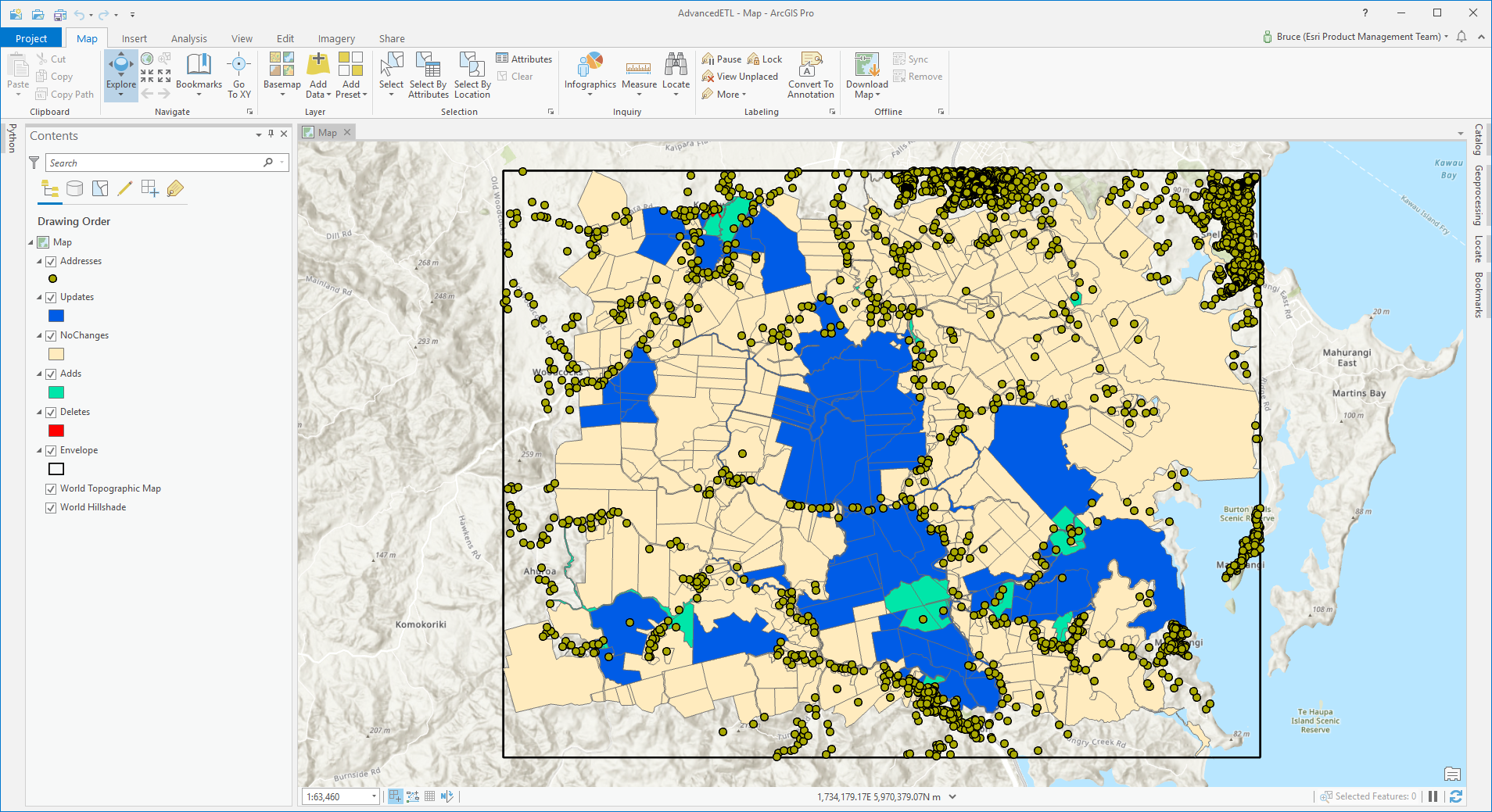
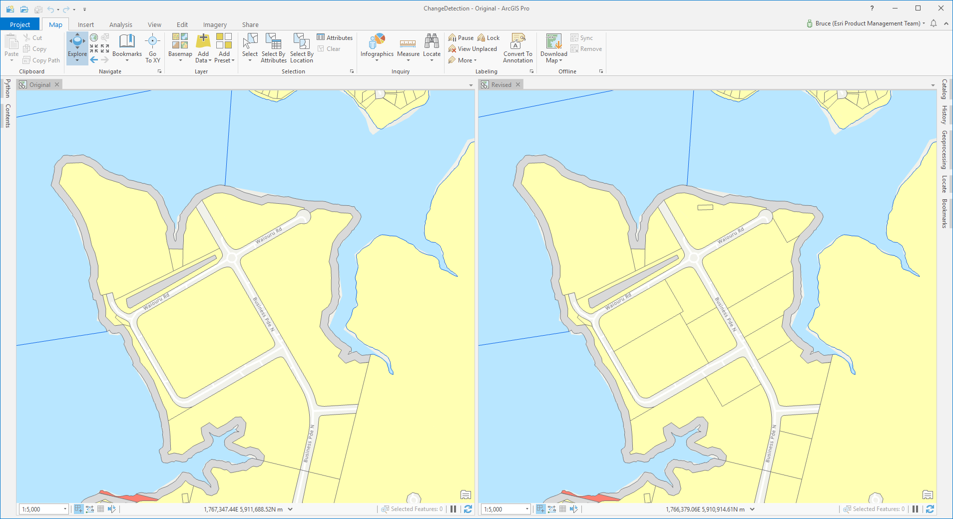
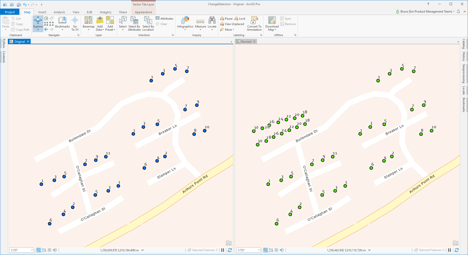
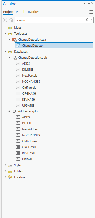
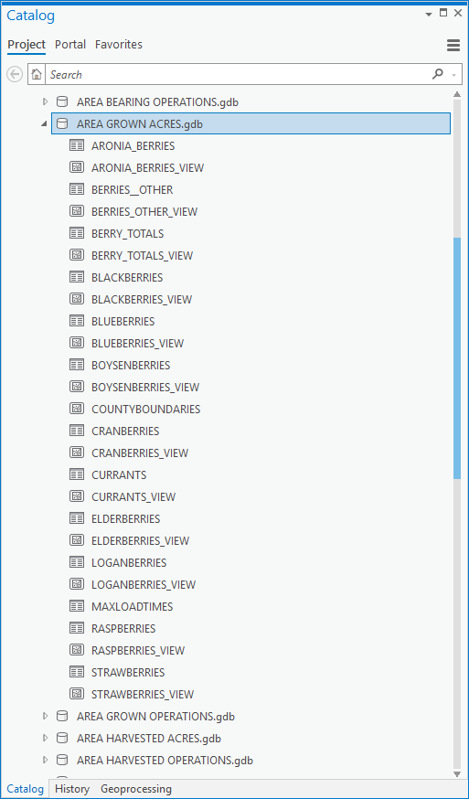
Expanding the 'AREA GROWN ACRES' dataset we can see the views, ready for use in a map:

Lets have a look at a view.  I'm going with peanuts.  I have never made a study of peanuts, but at least I know what they are.  Working with this data I learned of crops like Escarole Endive, which I may have eaten but never knew.  I like red-skinned Valencia peanuts, I think they make the best peanut butter, and to believe the packaging, excellent ones come from Texas.  I also buy a lot of peanuts in the shell (roasted, unknown variety, unsalted) to feed the wildlife in our yard, and that packaging assures me Virginia peanuts are great too.  Peanuts here we go.

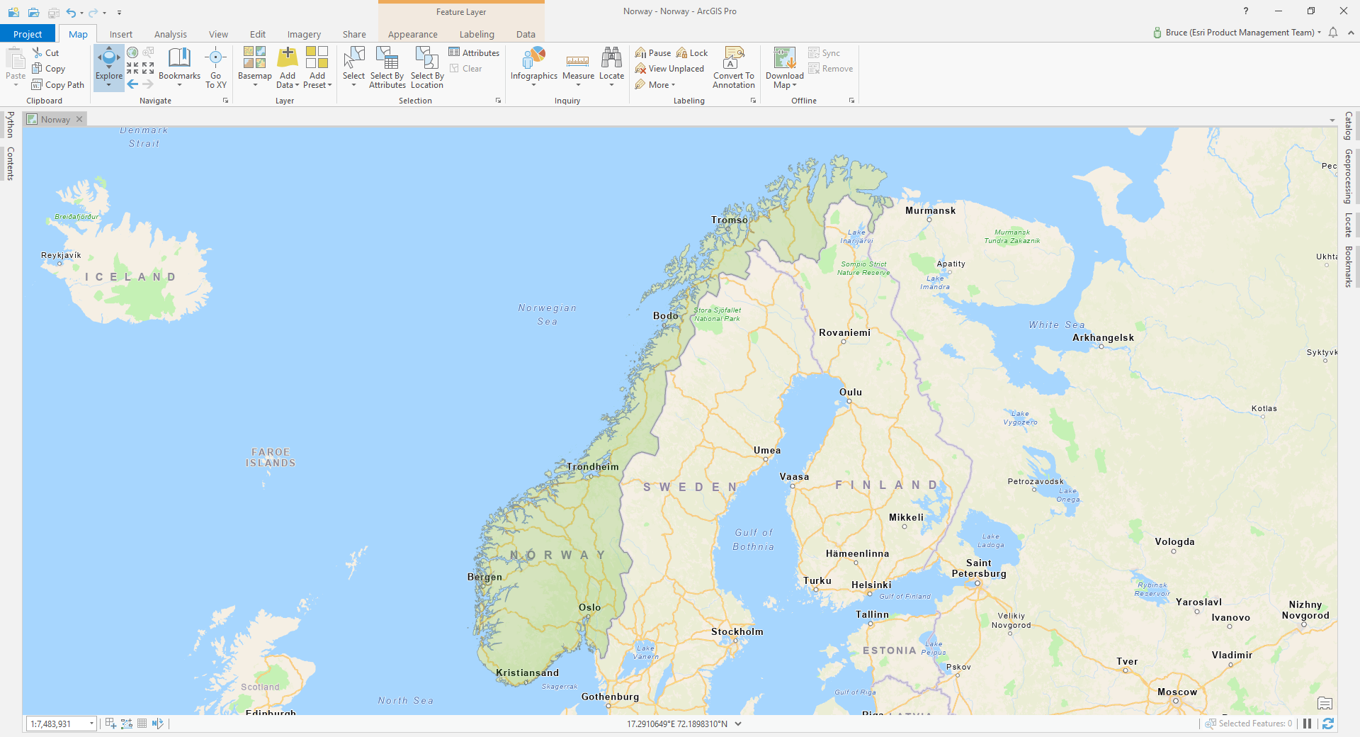
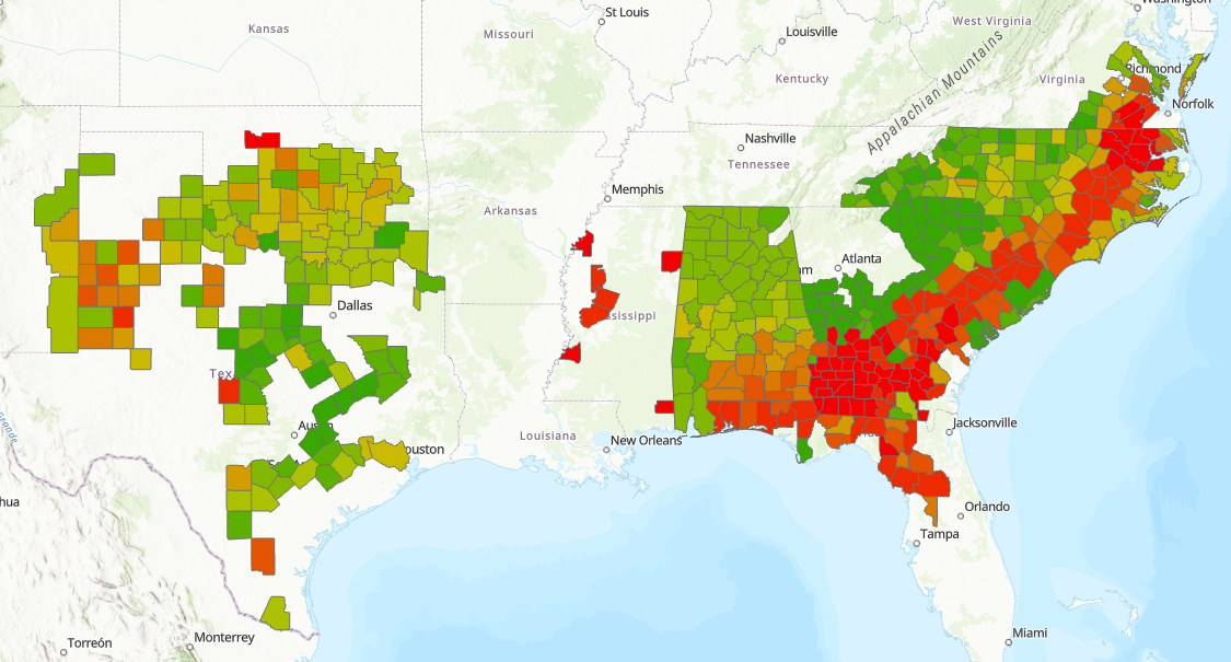
I added PEANUTS_VIEW from the workspace YIELD LB PER ACRE.gdb to my map and symbolized by VALUE with graduated color using 10 classes with a color ramp from green to red (red is high productivity).  Displaying all features I can see the engine room of peanut productivity is the arc of land across Mississippi, Alabama, Georgia, the Carolinas and up to Virginia, and more west of the Mississippi in Oklahoma and Texas.

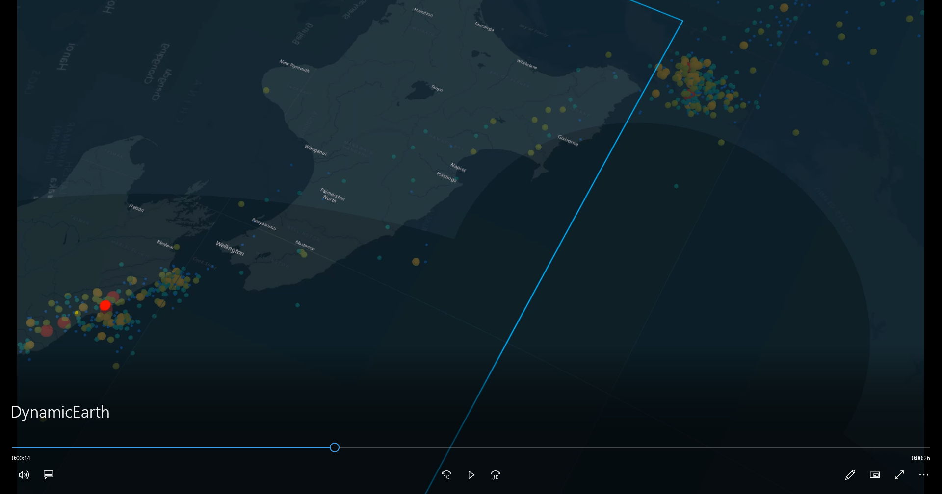
Time enabling on YEAR gives us the real story behind peanuts though.  In the download, view the 30 second movie PeanutsTheMovie.mp4.  This animates in single-year frames for all years 1934 to 2018.

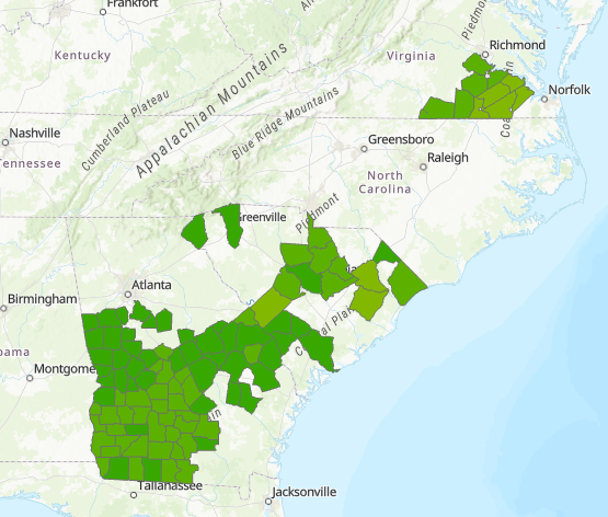
Here is 1934, what we might now call historically low yield and only in the east of 'peanut country':

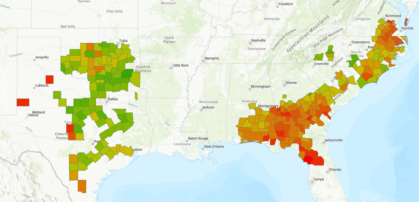
By 1965 productivity and range had increased:

By 1975 productivity and expansion had greatly increased:

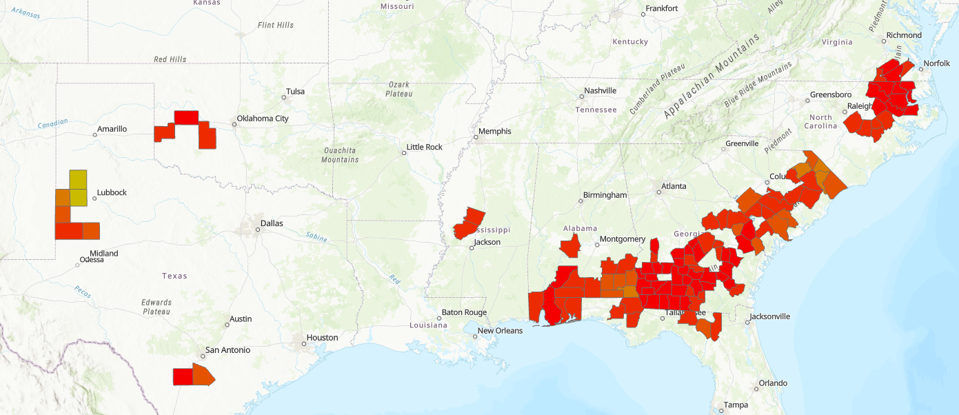
..and moving right along to the current time, peanut yield per acre has reached yields ten times historic values:

A common issue with big data is you want to find what has changed - what is new.  This is where the script tool ReportLoadTimes comes in.  This reads each MAXLOADTIMES table and emits a message about the most recent crop(s) statistic in each workspace.  For my data at time of writing I can see this:

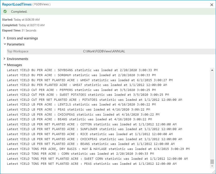
So for example in my workspace YIELD LB PER ACRE where my peanuts view lives, the latest statistics are for these crops updated a few days before finishing this blog:

Latest YIELD LB PER ACRE : LENTILS statistic was loaded at 4/16/2020 3:00:22 PM

Latest YIELD LB PER ACRE : PEAS statistic was loaded at 4/16/2020 3:00:22 PM

Latest YIELD LB PER ACRE : CHICKPEAS statistic was loaded at 4/16/2020 3:00:22 PM

Latest YIELD LB PER ACRE : BEANS statistic was loaded at 4/16/2020 3:00:22 PM

All crops sharing the latest load date are reported.

I hope this gives you confidence to tackle your own big data problems with ETL and File GDB views.  I read that for NASS data there are many commercial decisions made based on crop statistics and you will have your own business drivers.  Caveat:  NASS has some peculiarities that prevent all records displaying, for example some VALUE values are non-numeric and are discarded by this processing, and there are some county aggregations that cannot be mapped to county boundaries, so don't go building your peanut butter factory on my analysis.

Have fun!

A powerful feature of ArcGIS Data Interoperability and 'cousin' FME is the ability to save and share connections to web apps.  Once configured, you can use a web connection to read and write data in any number of workspaces while maintaining secure credentials in only one place.

Portal for ArcGIS is a component of ArcGIS Enterprise I think of as a content management system.  You can start reading about it here.  A portal is a highly capable, single-tenant, secure geospatial infrastructure component where you can create, maintain and share data, maps, scenes and apps.  This blog is about creating and using a portal app to access hosted feature services to be read and written with the ARCGISPORTALFEATURES reader/writer or the ArcGISOnlineConnector transformer.

The starting point is your portal, here is my portal's home page (fake, but you'll get the idea):

https://nonexistent.esri.com/portal/home/index.html 

The first thing to do is create an app to hang the web connection off.

Go to your Content view and click to Add Item:

Choose 'An application' and click Application and fill in the descriptive stuff:

The app will be created and you'll be taken to its home URL, which will look something like this:

https://nonexistent.esri.com/portal/home/item.html?id=50bfc12ef28840d48eac324c8ec67dd0 

In the top right is the Settings view, click on it.

Scroll down (or click on Application beside General top left) and you'll see App Registration:

Click on Registered Info to see details you'll need to create your web connection:

Click on Show Secret to expose the 32-character hex authentication key.  Now you have everything you need to create your portal web app connection for Workbench.  From the Pro Analysis ribbon (or by editing any ETL tool) open the Workbench application and go to Tools>FME Options>Web Connections.  Mine look like this (login obscured):

Click on Manage Services bottom right and in the Manage Web Services dialog use the pulldown bottom left to Create From and pull right and choose Esri ArcGIS Portal (Template).

Now fill in the dialog:

Test and Authenticate, then close the dialog, and you can add a web connection:

...and you are in business!

Restart Workbench and use the new web connection to add a portal feature service reader (login obscured):

Now enjoy your portal features ETL!

In an earlier post I introduced a technique for capturing map extents from user input and sending these as parameters to a Spatial ETL Tool.  This made the spatial extent of the processing dynamic with user input.  The key was wrapping the ETL tool with ModelBuilder to take advantage of its ability to interact with a map.

This post is along similar lines except showing how to capture a user's selection of feature classes to process at run time.  This makes the feature types being processed dynamic with user input.

First some background.  The FME Workbench application used for authoring Spatial ETL tools is designed for repeatable workflows with known input feature types, and the work centers around managing output feature characteristics.  In ArcGIS we are used to geoprocessing tools being at the center of data management and needing to handle whatever inputs come along.  We're going to make Spatial ETL a little more flexible like ArcGIS with some modest ModelBuilder effort.

Here is some data:

In my project database it looks like this (the main point is it is all in one geodatabase):

...and my Project Toolbox has a Spatial ETL Tool and a Model:

The Spatial ETL Tool...

...does absolutely nothing!  Well, it reads some default feature types from a default File Geodatabase, then writes them all out to the NULL format (great for demos, it never fails).  The trick here is I made the 'FeatureTypes to Read' input parameter of the File Geodatabase reader a User Parameter (you right click on any parameter to publish it this way).

The only other thing to 'know' ahead of the Modelbuilder stuff is that the ArcGIS Pro geoprocessing environment is smart enough to see Spatial ETL tool inputs and outputs that are Workspaces in geoprocessing terms (Geodatabases, Databases, Folders) as the correct variable type in ModelBuilder but that usually other FME Workbench workspace parameters you might expose are seen as String geoprocessing parameter type.  This means in our case if we choose multiple feature classes from my project home Geodatabase, like say 'Adds' and 'Deletes', then the ETL tool wants the value supplied to be a space-separated string like 'Adds Deletes'.

Here is the model, DynamicFeatureTypesModel.  Its last process is the Spatial ETL tool DynamicFeatureTypes.  There are three processes ahead of it.

On the left is the sole input parameter 'FeaturesToRead', of type Feature Class (Multi Value) (you could use Feature Layer too with a little more work in the model to retrieve source dataset paths):

There are three Calculate Value model tools, their properties are:

Get GDB:

This returns the Geodatabase of the first feature class in the input set.

GetFeaturesToRead:

This returns the names of the feature classes as a space-separated string.

GetGDB and GetFeaturesToRead supply the ETL tool input parameter values.

CheckSameWorkspace:

This returns a Boolean test that all input feature classes are from the same Geodatabase.  It is used as a precondition on the Spatial ETL Tool as that is designed with a File Geodatabase reader and must receive that format data and only once.

That's it!  The DynamicFeatureTypes model can be run like a normal project geoprocessing tool with the ability to select any desired inputs, and the Spatial ETL tool behind the scenes takes what it gets.  If you select inputs from different File Geodatabases the precondition check will prevent the tool from executing.

Here is the details view from a run with data from a different Geodatabase.

Please do comment in this blog with your comments and experiences.  The project toolbox and ETL source are in the post attachment.

Earthquakes definitely fall into the 'hard to see' category, but also tricky to get right in your GIS.

You can easily find earthquake data, government agencies offer feeds and historic databases from which you can extract data.  This is great for 2D maps, but often the Z (vertical) coordinates are given as positive depth values in kilometers, so 'going the wrong way' for the normal 'positive up' coordinate system.  Another wrinkle is the default Z domain for geodatabases has a Z minimum at -100,000, and the lithosphere extends below this depth in meters, so you can lose features on the way in.

I'm not going to do a big post on coordinate systems, I'm just going to throw a couple of things over the fence for you to look at.  Firstly watch the movie file in the blog downloads.  I was involved a few years ago in adjusting GIS data after an earthquake moved the ground (a lot, over 6m in some places).  Just watch the movie to see a year's worth of quakes go by and fly to where a lot of deformation occurred after a severe one; you'll fly past labels of movement values and to a homestead that shifted.  The apparent sudden jump of the property is real, and what you'll see is high resolution orthophotography before and after the adjustment work (it didn't have to be re-flown, just adjusted).

The movie was exported from an ArcGIS Pro 3D Scene, but this was only possible with correct 3D points for the quakes, and that data was made from a GeoJSON download and processing with the Spatial ETL tool Quakes2016.fmw that is the second download file.

Its a really simple workspace....

..until you go to the Tool Parameters>Scripting>Startup Script setting and see a bit of fancy footwork making a custom Feature Dataset in the output geodatabase with a Z domain that goes to the center of the earth.  The takeaways are you might not have known about startup scripts and that you can use one to operate on workspace parameters.

Please comment on the post with your experiences and ideas.

Dataset management in ArcGIS has plenty of supporting tools and workflows, but when you don't have control for any reason you may be the person who has to figure out what data changed, and where.

This blog is about a tool published in the ArcGIS Online sample galleries for bulk change detection between pairs of feature classes.

My first example datasets are two parcel feature classes, where one has been revised with survey and subdivision work, but without any edit tracking fields - the data is not managed in ArcGIS.  The maps are named for their content, Original has the old data, Revised has the new data.

The two datasets have about 650,000 features each over a huge area, so visual comparison is impossible, especially as I need to compare attributes too.  The Feature Compare geoprocessing tool is an option if my data has a unique key field to sort on (it does) but its output is a table, I want features.

The Pro Change Detector tool delivers flexible change detection between two feature classes with your choice of attribute and geometry comparison, and outputs feature classes of Adds, Deletes, Updates and NoChanges (Updates are only detectable if the data has a unique key field separate to ObjectID; without a key field updates are output as spatially overlapping deletes and adds).

The tool requires the ArcGIS Data Interoperability extension, but you don't have to learn to drive the Workbench application delivered with Data Interoperability, this sample is just a normal Python script tool.

For my parcel data I chose all the attributes to be considered as well as geometry:

Then 7 1/2minutes later after comparing ~650,000 features per input I had my change sets:

You can compare any geometry type but if you are going to do change detection of multiple pairs of feature classes be sure to change the output objects names as the tool will overwrite its outputs.  Alternatively, keep your data in separate project databases (see below).

For a second example I decided to 'go big' and compare two street address datasets each with about 2 million features and a lot of attributes:

Now its 22 minutes to find a couple of thousand changes to 2 million features:

...and in the map it is easy to find a locality where subdivision has resulted in new addresses being created - see the extra address points in the Revised map:

To use the tool your data must be in a single File Geodatabase, here is how my Catalog pane looks, note to preserve my change sets I used two separate databases in the Project.

The tool was created with ArcGIS Pro 2.5 beta 2 software (sharp eyed people will see the new style geoprocessing Details view above) but works in Pro 2.4.  You will need ArcGIS Data Interoperability installed and licensed, and you'll need permission to copy a file into the install of your Pro software, please see the README file in the download.

Now go detect some changes and comment in this blog how you get on!

Edited 2/8/2021 to replace the .pth file with one suitable for Python 3.7 in Pro 2.7+

Many organizations publish OGC WFS services as one option for data supply, either to the general public or to a restricted audience.  Often however these services are intended for large scale mapping, such as within a single municipality, and bulk download at national scale is not supported - either a maximum feature collection size per request is set on the server, or response paging is not supported, so an out-of-the-box client is not going to deliver an entire dataset.   Sometimes, although these restrictions are not present, assembling and delivering a request for a large feature collection is beyond the capability of the server or network settings (by design), or the client app doesn't support paging (full disclosure, WFS 2.0.0 response paging is coming to core ArcGIS Pro in a future release; Data Interoperability extension already supports WFS 2.0.0 paging if the server provides next/previous URLs).

This blog is about using ArcGIS Data Interoperability to work around these limitations to achieve repeatable bulk download of WFS data at any scale.  You will need solid Data Interoperability (or FME) skills to implement this workflow, or be willing to learn from the content of the blog download.

At this point I need to show you a map or you'll go do something else, so I bring you today's subject matter - Norway!

It's necessary to use a real world example, and the people at GeoNorge have excellent public WFS services that let me show the issues, so Norway is it.  Browsing their site I settled on a road network service.  Here is how to get there yourself, while optionally learning a little Norwegian.  Here is GeoNorge, (don't use '/en' if your Norwegian is up to it) click on Go to the map catalogue, then in the selector pane on the left choose Type = Service, Topic = Transportation, Distribution form = WFS Service, then of the available services click on ELF Road Transport Network.  Scroll down and you'll see:  Get Capabilites Url: https://wfs.geonorge.no/skwms1/wfs.inspire-tn-ro?request=GetCapabilities&service=WFS.

• Run ReadWFSFeatures.fmw with a WHERE clause selecting the smallest cell size (initially Shape_Length = 400000, then 200000 when those cells are made, then 100000 when those are made in a subsequent step below...)
• Add the output RoadLink feature class to your map
• Run RoadCount.py in the Python window to populate RoadCount in NO_Fishnet
• Select NO_Fishnet features with RoadCount >= 9000 (undershooting 10,000 to allow for road construction)
• If there are no NO_Fishnet features selected then BREAK - you are finished making the fishnet
  
• Run MinimumBoundingFishnet to create a separate fishnet with cells half the width/height of the previous minimum; it is important the selection on NO_Fishnet is still active
• Run Delete Features on the selected NO_Fishnet cells
• Run Append to add the generated smaller fishnet cells to NO_Fishnet, using the field map option.
• Run SetExtentAttributes.py in the Python window to recalculate the boundary coordinates
• Delete the RoadLink feature class
• Go back to the first step

The National Emergency Number Association promulgates GIS standards for datasets that support public safety operations in the USA.  A principal example is Civic Location Data Exchange Format (CLDXF).  Digging in further we can find a well defined data model for address points. The problem we're tackling in this blog is how to directly use data maintained in this schema to create ArcGIS geocoding locators without anyone having to construct complex ETL processes and copy data around repetitively.

The workflow requires your NENA data be maintained in an Enterprise Geodatabase, and there is a disclaimer - the full granularity of subaddress elements in the NENA schema is not supported.  At time of writing (Pro 2.4.1 release) only one pair of subaddress type & identifier values is supported, but the sample demonstrates how three pairs of type & identifier values can be handled, as at the Pro 2.5 release locators will support this many subaddress fields.  My test data (the counties of Kings, Queens, Nassau and Suffolk in New York, thanks to NYS GIS Clearing House) has units (apartments etc.), levels (floors, basements etc.) and building units (rooms, annexes etc.).  Building name is usable too, and seat in the room and additional location data is retained and may be output by a locator but not used for searching.

Before we go further, why doesn't Esri just design the Create Locator tool to accept all the NENA fields?  The short answer is we have to have internationally applicable parameters so it would overload the tool.

I said 'no ETL required'.  Well hopefully that is true for you, and for my test data it would be if I had access to the database, but what I often see in the wild is things like empty strings and blank values in character fields, so I like to enforce proper null values and fix invalid date values with a bit of processing with Data Interoperability extension.  In the screen captures below (click on images to enlarge) I'm making sure empty data is null as I import my test data to my EGDB.

The only other thing I did with my ETL was rename fields to lower case (what PostgreSQL likes, my EGDB platform) and make a couple of fields wider (pretype, posttype) in case my concatenations overflow those fields.  Make sure domains don't bite you too, you'll be adding new values to pretype and posttype fields.  Having said that though, I see in the data view of my layer that the character fields have arbitrary widths of 255 characters, so I'm not sure if the input field definitions are honored, or that views have any concept of domains, this is something that might be platform dependent.  Anyway, that gets me to what should be your starting point.  I have NENA-schema address points in my EGDB and I want to make a locator.

The secret sauce here is creating a view in my DBMS that performs all the manipulations necessary to rename, cast, substring and concatenate data into a schema directly usable in ArcGIS Pro as a feature layer input to the Create Locator geoprocessing tool, using the Point Address data role.

I seldom descend into SQL to this depth so to develop my view I built it up in pgAdmin (you'll need whatever SQL authoring tool comes with your DBMS), going field by field and inspecting the result in Pro as I went.  Tip:  you can recreate your view in pgAdmin and leave it in Pro's table of contents and just reset the layer source each time you want to view it - it will refresh in the map.

The blog download has the pgAdmin SQL source - esri_view.sql - and you can inspect the comments to understand the logic.  Basically the fields specific to NENA that cannot be mapped to Point Address role inputs have their values passed into other fields.  Fields combining type & identifier values are parsed into separate fields for each.  The SQL will need to be ported to your environment, but its pretty standard stuff.

If you are a SQL wizard and can go straight to a SELECT statement then you could use the Create Database View tool and input the view definition.  The edited source (no comments in it) is the file test_view.sql in the download.  No prizes for user interface design but it works:

Having created the view, add it to your map and specify the ObjectID field as the unique identifier:

Let it index and you have your (dynamic) view of NENA data in your map as a feature layer:

You can see why I had to widen the type fields, check out '1375 Sunrise Hwy Westbound Service Road, Islip, NY, 11706'

Anyway, run Create Locator (hard to make an exciting graphic but hopefully useful):

arcpy.geocoding.CreateLocator("USA", "nena.sde.esri_view PointAddress", @"""PointAddress.ADDRESS_JOIN_ID 'nena.sde.esri_view'.address_id"";""PointAddress.HOUSE_NUMBER 'nena.sde.esri_view'.house_number"";""PointAddress.BUILDING_NAME 'nena.sde.esri_view'.building_name"";""PointAddress.STREET_NAME_JOIN_ID 'nena.sde.esri_view'.street_id"";""PointAddress.STREET_PREFIX_DIR 'nena.sde.esri_view'.prefix_direction"";""PointAddress.STREET_PREFIX_TYPE 'nena.sde.esri_view'.prefix_type"";""PointAddress.STREET_NAME 'nena.sde.esri_view'.street_name"";""PointAddress.STREET_SUFFIX_TYPE 'nena.sde.esri_view'.suffix_type"";""PointAddress.STREET_SUFFIX_DIR 'nena.sde.esri_view'.suffix_direction"";""PointAddress.SUB_ADDRESS_UNIT 'nena.sde.esri_view'.unit"";""PointAddress.SUB_ADDRESS_UNIT_TYPE 'nena.sde.esri_view'.unit_type"";""PointAddress.NEIGHBORHOOD 'nena.sde.esri_view'.neighborhood"";""PointAddress.CITY 'nena.sde.esri_view'.city"";""PointAddress.METRO_AREA 'nena.sde.esri_view'.metro_area"";""PointAddress.SUBREGION 'nena.sde.esri_view'.county"";""PointAddress.REGION 'nena.sde.esri_view'.state"";""PointAddress.POSTAL 'nena.sde.esri_view'.zipcode"";""PointAddress.COUNTRY 'nena.sde.esri_view'.country""", r"C:\Work\Product_Management\Address_Management\Nena", "ENG", None, None, None)

Then geocode!

Units work:

285 Asharoken Ave, #1, Huntington, NY, 11768

Fancy house numbers work:

5 1/2 Locust Ave, Brookhaven, NY, 11790

Building names work:

Building 22A, John F Kennedy Airport, New York, NY, 11430

So there you have it, maintain your data in NENA compliance and use it to geocode.

But wait, there's more!  In response to the blog commentary around handling aliasing the download has been updated to add the SQL source esri_views.sql that creates an alternate city name table, used as below in Create Locator - see the Alternate Name Tables section:

Ignore the warning chip in the dialog capture, that just appears after locator creation to indicate you'll overwrite the output if you re-run the tool.

The wisdom of harvesting alternate city names from as many fields as i did can be debated, but hopefully you get the idea, the various NENA fields for zone values can be viewed suitably for use as alternate name roles.  In production, it would be more efficient to create an alternate city name table from centerline data and join to it on street_id.

Here is the view used as the alternate city name table:

The address with address_id = 'KIN0000001' is '463 Maspeth Ave, New York, NY, 11211'  Using the city alias 'Brooklyn' works with score = 100:

Additionally, I took a question off-line about maintaining all parts of addresses defined in the FGDC standard such as prefix and suffix address number parts, street name separator elements, pre-modifiers and post-modifiers.  If you want to output these elements when geocoding then define them as custom output fields for your locators.  This functionality is available in the tool as the last parameter, but you'll also need to supply source fields in the field map for each output.

I output seat and additional_location in my locator, which would let me work on candidates if that's what I needed.

GeoNet Ideas contains many customer requests for ODBC connectivity from Pro to databases that are not supported ArcGIS workspaces.  This blog is about implementing read-only import of ODBC data sources to Geodatabase.  See also the paragraph titled 'Update' for a simple way to move data sources between formats using the same underlying approach.

Thumbnail:  We'll use a scripted approach, creating a Python script tool in a Pro toolbox.  You could make this a standalone script and a scheduled task.  The coding isn't scary.  You'll need permission to create an ODBC data source on your computer, and if you need to publish this to ArcGIS Enterprise the data source will need to be set up there too.  If multiple users need to use the tool on your machine the ODBC data source will need to be a system one.  Off we go...

The ArcGIS Pro python environment ships with a module named osgeo, from the OSGeo organization.  This supplies the GDAL libraries that support conversion of hundreds of geospatial formats, and one of the supported sources is ODBC, which isn't a 'format' of course but handles moving tabular data around.

For my example source I chose MariaDB, a binary equivalent to MySQL.  After installing MariaDB and the appropriate 64bit ODBC driver I imported some CSV data and created a user-level ODBC data source in Windows.  Here is how the admin tool looks (click on images to enlarge them):

MariaDB ships with a handy administration utility - HeidiSQL - here is how the Data view of my target data looks in HeidiSQL (the names and addresses are made up):

So that's my target data, now how to get at it?  To understand what the osgeo module needs to connect to my ODBC source I researched the relevant vector driver.  So far so good.  With a little more surfing some examples and the submodule osgeo.ogr API the parts were apparent.  Next step - code it!  Here is the result in my project:

The blog download has the tool and source, plus the CSV data I used.  Disclaimer: this is a very simple example without any defensive code to handle variability in the input data.  The idea is to give you confidence you can script a repeatable workflow.

How did I do?   I run the tool:

...and the output table is created in my project home geodatabase.

Success!  I imported 6000 rows in about 8 seconds.  So that is the pattern I wanted to show.  The approach will handle more data types than just the string and integer values I used, and it is quite likely the part of my code where I map OGR field types to ArcGIS field types has issues.  Please do comment in this blog space on your challenges and successes.

Now for the optional extra - Access databases!

I have 64bit Office on my machine, I also have Microsoft Access Runtime 2013 installed, I'm not entirely sure if both are needed or just one but my ODBC datasource options include .mdb and .accdb.  Otherwise the pattern to reading Access databases is the same as the above.  I configured an ODBC MS Access Database connection in the 64bit ODBC administrator to connect to an .accdb database on disk.  I possibly should have added a new one and given it a descriptive name but you get the idea.  From there it is just like any other ODBC source, except it does have a dependency on 64bit Office and/or the runtime driver.

Update:  I created this sample with a rudimentary knowledge of what the OGR drivers delivered with the osgeo module can do.  It is way easier to just copy an OGR layer to an OpenFileGDB layer than create one with ArcPy and use a cursor to write into a new table or feature class.  Re-purpose the approach I describe in the comments in the below post about the OpenFileGDB driver:

https://community.esri.com/ideas/15746 

Everyone likes SQLite. It is a single portable file, performs and scales well, supports enough SQL to be useful and has a DB-API compliant Python module and API access in other languages. It is embedded in many mobile and desktop apps, and is directly usable in ArcGIS Pro.

SQLite as a container has an incarnation - OGC GeoPackage - that supports the encoding of vector and raster features for direct use in ArcGIS Pro.  You can read about the standard on the OGC website.

The GIS format most often compared with GeoPackage is the Esri-defined shapefile.  Shapefile is the most shared GIS format on the planet and its encoding of vector features is published.  Note however the publication date - 1998.  At the time the shapefile was designed, the components available had limitations that can frustrate today's advanced workflows.  These include file size limit, attribute field count and name width limits, dates not supporting time, complexity in handling character encodings and lack of null value support for most field types.  Shapefile has been spectacularly successful for handling simple vector features, but it can be limiting.

I think of GeoPackage as the new shapefile without the old limitations and I encourage you to use it. It is a great format for, well, geo-packaging! However, don't go as far as thinking it is a full-blown GIS workspace, it doesn't have geodatabase behaviors like domains and attribute rules. What it does, it does well.

GeoPackage is extensible, and there are approved OGC extensions for gridded tiles of elevation data and table relationships, and non-approved community extensions such as map styling of features and storing vector tiles. ArcGIS Pro does not yet implement support for any GeoPackage extensions (excepting table functionality adopted in the v1.2 release).

What can you do with a GeoPackage in ArcGIS Pro 2.6?

• Read and write simple features (polygons, polylines, points, multipoints, circular arcs, tables)
• Create feature classes with the Feature Class to Feature Class tool
• Create tables with the Table to Table tool
• Use Copy/Paste in the Catalog pane
• Use the Append tool to add data to an existing feature class or table
• Use the Add Raster To Geopackage tool to store imagery

• Edit features or rows with the ability to undo and redo edits

• Modify the schema
• Geoprocess with any tool that takes a simple feature class or table as input
• Share GeoPackage data with other users as a static item in ArcGIS Online
• Use Geopackage  vector and raster data in map workflows
• Read or write GeoPackage in Data Interoperability ETL workflows
• Use SQL statements in SQLite's native dialect

What can you not do with a GeoPackage in ArcGIS Pro 2.6?

• Publish a GeoPackage item as a hosted web layer
• Store or edit metadata
• Use any geoprocessing tool that requires geodatabase output

Some recommendations:  You can add fields and calculate values with geoprocessing tools or ArcPy, but you may find it slower than native geodatabase operations.  Geometry storage in a GeoPackage is not compressed like a geodatabase, so they can get big.  Do your geoprocessing before creating your GeoPackage, then copy your data into it.  Think of GeoPackage as a sharing format.

Move your data into the GeoPackage like this:

• Create a GeoPackage with the Create SQLite Database tool (using the GeoPackage spatial type)
• Use the Copy tool (Data Management, General toolset) to add vector data, or Copy/Paste in the Catalog pane
• Use the Add Raster to GeoPackage tool (Conversion, To GeoPackage toolset) to add raster mosaics

Your GeoPackage is now ready for use.

Note on sharing:  You can upload a .gpkg file to ArcGIS Online, the file type will be recognized.  You can send a link after sharing the item and others can then download it from the content gallery.

Advanced topic:  Because it is based on SQLite, GeoPackage comes with a database engine and good SQL language support.  There are 3rd party tools for working with SQLite which you may find useful, but to include a spatial component in your work the ArcGIS Data Interoperability or Safe Software FME products support scripting SELECT, CREATE, DROP, DUPLICATE, TRUNCATE and CROSS JOIN statements within Spatial ETL tool transformers like SQLCreator and SQLExecutor.  This approach enables very powerful and performant use of a GeoPackage.