Python Blog - Page 14

cancel
Showing results for 
Show  only  | Search instead for 
Did you mean: 

Latest Activity

(198 Posts)
DanPatterson_Retired
MVP Emeritus

Snips of interest...

: -----------------------------------------------------------------------------------------------------------------------------------------------------------

Update... Guarantee ordered dict literals in v3.7?

Guido van Rossum guido at python.org
Fri Dec 15 10:53:40 EST 2017

Make it so. "Dict keeps insertion order" is the ruling. Thanks!

Dictionary order? without 'ordered dictionaries' ?  Not in 2.x... nope!  You had to use ordered dictionaries, but what about dictionaries? How about they are 25% faster than in 2.7... interested now

k = list('abcd')
v = [1,2,3,4,5]
dct = {k:v for k,v in zip(k, v)}

dct
{'a': 1, 'b': 2, 'c': 3, 'd': 4}‍‍‍‍‍‍‍‍‍‍‍‍‍‍‍‍‍‍‍‍‍‍‍‍‍‍‍‍‍‍‍‍‍‍

Loads of other tidbits.... What's new in Python 3.6

  • math.tau... cmath.tau, cmath.inf and cmath.nan to match math.inf and math.nan, and also cmath.infj
    • Still haven't a use for tau? infinity? not a number? imaginary complex numbers????  Now is your chance to get a foot up on the others.
  • json.load() and json.loads() now support binary input, json is still ugly, but in binary it won't matter cause you can't read it anyway
  • os and os.path modules now support path-like objects.  This isn't what forgetting to put the important stuff in front of the filename by the way.
  • pathlib now supports path-like objects.  Never heard of pathlib?  Read up.
  • statistics... now has a harmonic mean.  I bet you didn't even know that there was a statistics module did you?

: ------------------------------------------------------------------------------------------------------------------------------------------------------

Abandon ship... Supporters have begun to announce when the last call from port is

This is a biggie, since so many other science packages depend on it.  SciPy is in discussions as well.  Maybe you-know-who will also announce similar plans

Sunset time... The exit time and supporters list  The list is growing...

Belated Happy 8th python...  Grown quite a bit over the intervening 8 years.  

What is new in Python 3.7.... you are growing so fast

This blog-ette is just to show some things that should be used more in python 3.x.  Sadly... they aren't even available in python 2.7.x.  (The party is going to be delayed for ArcMap 10.5)

I often work with lists and array and tabular data, often of unknown length.  If I want to get the 3rd element in a list or array or table, you can do the old slicing thing which is fine.  

  • But what if you only want the first two but not the rest?
  • What about the last 2 but not the rest?  
  • How about the middle excluding the first or last two?  
  • How about some weird combination of the above.
  • What if you a digital hoarder and are afraid to throw anything away just in case...

Yes slicing can do it.  What if you could save yourself a step or two?.

To follow along... just watch the stars... * ... in the following lines.  I printed out the variables all on one line so they will appear as a tuple just like usual.  Now when I say 'junk', I mean that is the leftovers from the single slices.  You can't have two stars on the same line, before I forget but you can really mess with your head by parsing stacked lines with variable starred assignment.  

Let's keep it simple ... an array (cause I like them) ... and a list as inputs to the variable assignments... 

>>> import numpy as np
>>> a = np.arange(10)
>>>
>>> # ---- play with auto-slicing to variables ----
>>> a0, a1, *a2 = a       # keep first two, the rest is junk
>>> a0, a1, a2
(0, 1, [2, 3, 4, 5, 6, 7, 8, 9])

>>> a0, a1, *a2, a3 = a   # keep first two and last, junk the rest
>>> a0, a1, a2, a3
(0, 1, [2, 3, 4, 5, 6, 7, 8], 9)

>>> *a0, a1, a2, a3 = a   # junk everything except the last 3
>>> a0, a1, a2, a3
([0, 1, 2, 3, 4, 5, 6], 7, 8, 9)

>>> # ---- What about lists? ----
>>> *a0, a1, a2, a3 = a.tolist()  # just convert the array to a list]
>>> a0, a1, a2, a3
([0, 1, 2, 3, 4, 5, 6], 7, 8, 9)

‍‍‍‍‍‍‍‍‍‍‍‍‍‍‍‍‍‍‍‍‍‍‍‍‍‍‍‍‍‍‍‍‍‍‍‍‍‍‍‍‍‍‍‍‍‍‍‍‍‍‍‍‍‍‍‍‍‍‍‍‍‍‍‍‍‍‍‍‍‍‍‍‍‍‍‍‍‍‍‍‍‍‍‍‍‍‍‍‍‍‍‍‍‍‍‍‍‍‍‍‍‍‍‍‍‍‍‍‍‍‍‍‍‍‍‍‍‍‍‍‍‍‍‍‍‍‍‍‍‍‍‍‍‍‍‍‍‍‍‍‍‍‍‍‍‍‍‍‍‍‍‍‍‍‍‍‍‍‍‍‍‍‍‍‍‍‍‍‍‍‍‍‍‍‍‍‍‍‍‍‍‍‍‍‍‍‍‍‍‍‍‍‍‍‍‍‍‍‍‍‍‍‍‍‍‍‍‍‍‍‍‍‍‍‍‍‍‍‍‍‍‍‍‍‍‍‍‍‍‍‍‍‍‍‍‍‍‍‍‍‍‍‍‍‍‍‍‍‍‍‍‍‍‍‍‍‍‍‍‍‍‍‍‍‍‍‍‍‍‍‍‍‍‍‍‍‍‍‍‍‍‍‍‍‍‍‍‍‍‍‍‍‍‍‍‍‍‍‍‍‍‍‍‍‍‍‍‍‍‍‍‍‍‍‍‍‍‍‍‍‍‍‍‍‍‍‍‍‍

Dictionaries too.... but this example is so python 3.5..... look way up at the top of the page

>>> k = list('abcd')
>>> v = [1,2,3,4,5]
>>> dct = {k:v for k,v in zip(k, v)}  # your dictionary comprehension
{'c': 3, 'b': 2, 'a': 1, 'd': 4}

>>> # ---- need to add some more ----
>>> dct = dict(f=9, g=10, **dct, h=7)
>>> dct
{'h': 7, 'c': 3, 'b': 2, 'a': 1, 'g': 10, 'f': 9, 'd': 4}‍‍‍‍‍‍‍‍‍‍‍‍‍‍‍‍‍‍‍‍‍‍‍‍‍‍‍‍‍‍‍‍‍‍‍‍‍‍‍‍‍‍‍‍‍‍‍‍‍‍‍‍‍‍‍‍‍‍‍‍‍‍‍‍‍‍‍‍‍‍‍‍‍‍‍‍‍‍‍‍‍‍‍‍‍‍‍‍‍‍‍‍‍‍‍‍‍‍‍‍‍‍‍‍‍‍‍‍‍‍‍‍‍‍‍‍‍

Think about the transition to 3?

Update (2017-03)

Pro 2.0 uses python 3.5.3, hopefully the next release will use python 3.6 since it is already out and 3.7 is in development.

ArcMap will catchup, but I suspect not at the same rate/pace as PRO.

References

Python 3.0 Release | Python.org Happy Birthday Python

Python 2.7 Countdown 

For more examples far more complex than the above, see...

python 3.x - Unpacking, Extended unpacking, and nested extended unpacking - Stack Overflow 

more
1 1 1,349
DanPatterson_Retired
MVP Emeritus

So ... new interface, time to try out some formatting and stuff.  What a better topic than how to order, structure and view 3D data like images or raster data of mixed data types for the same location or uniform data type where the 3rd dimension represents time.


I will make it simple.  Begin with 24 integer numbers and arange them into all the possible configurations in 3D.  Then it is time to mess with your mind and show you how to convert from one arrangement to another.  Sort of like Rubic's Cube, but simpler.

So here is the generating script (note the new cool python syntax highlighting... nice! ... but you still can't change the brownish background color, stifling any personal code preferences).  The def just happens to be number 37... it has no meaning, just 37 in a collection of functions

def num_37():
    """(num_37) playing with 3D arrangements... 
    :Requires:
    :--------
    :  Arrays are generated within... nothing required
    :Returns:
    :-------
    :  An array of 24 sequential integers with shape = (2, 3, 4)
    :Notes:
    :-----
    :  References to numpy, transpose, rollaxis, swapaxes and einsum.
    :  The arrays below are all the possible combinations of axes that can be 
    :  constructed from a sequence size of 24 values to form 3D arrays.
    :  Higher dimensionalities will be considered at a later time.
    :
    :  After this, there is some fancy formatting as covered in my previous blogs. 
    """
    nums = np.arange(24)      #  whatever, just shape appropriately
    a = nums.reshape(2,3,4)   #  the base 3D array shaped as (z, y, x) 
    a0 = nums.reshape(2,4,3)  #  y, x axes, swapped
    a1 = nums.reshape(3,2,4)  #  add to z, reshape y, x accordingly to main size
    a2 = nums.reshape(3,4,2)  #  swap y, x
    a3 = nums.reshape(4,2,3)  #  add to z again, resize as befor
    a4 = nums.reshape(4,3,2)  #  swap y, x
    frmt = """
    Array ... {} :..shape  {}
    {}
    """
    args = [['nums', nums.shape, nums],
            ['a', a.shape, a], ['a0', a0.shape, a0],
            ['a1', a1.shape, a1], ['a2', a2.shape, a2],
            ['a3', a3.shape, a3], ['a4', a4.shape, a4],
            ]
    for i in args:
        print(dedent(frmt).format(*i))
    return a
‍‍‍‍‍‍‍‍‍‍‍‍‍‍‍‍‍‍‍‍‍‍‍‍‍‍‍‍‍‍‍‍‍‍‍‍‍‍‍‍‍‍‍‍‍‍‍‍‍‍‍‍‍‍‍‍‍‍‍‍‍‍‍‍‍‍‍‍‍‍‍‍‍‍‍‍‍‍‍‍‍‍‍‍‍‍‍‍‍‍‍‍‍‍‍‍‍‍‍‍‍‍‍‍‍‍‍‍‍‍‍‍‍‍‍‍‍‍‍‍‍‍‍‍‍‍‍‍‍‍‍‍‍‍‍‍‍‍‍‍‍‍‍‍‍‍‍‍‍‍‍‍‍‍‍‍‍‍‍‍‍‍‍‍‍‍‍‍‍‍‍‍‍‍‍‍‍‍‍‍‍‍‍‍‍‍‍‍‍‍‍‍‍‍‍‍‍‍‍‍‍‍‍‍‍‍‍‍‍‍‍‍‍‍‍‍‍‍‍‍‍‍‍‍‍‍‍‍‍‍‍‍‍‍‍‍‍‍‍‍‍‍‍‍‍‍‍‍‍‍‍‍‍‍‍‍‍‍‍‍‍‍‍‍‍‍‍‍‍‍‍‍‍‍‍‍‍‍‍‍‍‍‍‍‍‍‍‍‍‍‍‍‍‍‍‍‍‍‍‍‍‍‍‍‍‍‍‍‍‍‍‍‍‍‍‍‍‍‍‍‍‍‍‍‍‍‍‍‍‍‍‍‍‍‍‍‍‍‍‍‍‍‍‍‍‍‍‍‍‍‍‍‍‍‍‍‍‍‍‍‍‍‍‍‍‍‍‍‍‍‍‍‍‍‍‍‍‍‍‍‍‍‍‍‍‍‍‍‍‍‍‍‍‍‍‍‍‍‍‍‍‍‍‍‍‍‍‍‍‍‍‍‍‍‍‍‍‍‍‍‍‍‍‍‍‍‍‍‍‍‍‍‍‍‍‍‍‍‍‍‍‍‍‍‍‍‍‍‍‍‍‍‍‍‍‍‍‍‍‍‍‍‍‍‍‍‍‍‍‍‍‍‍‍‍‍‍‍‍‍‍‍‍‍‍‍‍‍‍‍‍‍‍‍‍‍‍‍‍‍‍‍‍‍‍‍‍‍‍‍‍‍‍‍‍‍‍‍‍‍‍‍‍‍‍‍‍‍‍‍‍‍‍‍‍‍‍‍‍‍‍‍‍‍‍‍‍‍‍‍‍‍‍‍‍‍‍‍‍‍‍‍‍‍‍‍‍‍‍‍‍‍‍‍‍‍‍‍‍‍‍‍‍‍‍‍‍‍‍‍‍‍‍‍‍‍‍‍‍‍‍‍‍‍‍‍‍‍‍‍‍‍‍‍‍‍‍‍‍‍‍‍‍‍‍‍‍‍‍‍‍‍‍‍‍‍‍‍‍‍‍‍‍‍‍‍‍‍‍‍‍‍‍‍‍‍‍‍‍‍‍‍‍‍‍‍‍‍‍‍‍‍‍‍‍‍‍‍‍‍‍‍‍‍‍‍‍‍‍‍‍‍‍‍‍‍‍‍‍‍‍‍‍‍‍‍‍‍‍‍‍‍‍‍‍‍‍‍‍‍‍‍‍‍‍‍‍‍‍‍‍‍‍‍‍‍‍‍‍‍‍‍‍‍‍‍‍‍‍‍‍‍‍‍‍‍‍‍‍‍‍‍‍‍‍‍‍‍‍‍‍‍‍‍‍‍‍‍‍‍‍‍‍‍‍‍‍‍‍‍‍‍‍‍‍‍‍‍‍‍‍‍‍‍‍‍‍‍‍‍‍‍‍‍‍‍‍‍‍‍‍‍‍‍‍‍‍‍‍‍‍‍‍‍‍‍‍‍‍‍‍‍‍‍‍‍‍‍‍‍‍‍‍‍‍‍‍‍‍‍‍‍‍‍‍‍‍‍‍‍‍‍‍‍‍‍‍‍‍‍‍‍‍‍‍‍‍‍‍‍‍‍‍‍‍‍‍‍‍‍‍‍‍‍‍‍‍‍‍‍‍‍‍‍‍‍‍‍‍‍‍‍‍‍‍‍‍‍‍‍‍‍‍‍‍‍‍‍‍‍‍‍‍‍‍‍‍‍‍‍‍‍‍‍‍‍‍‍‍‍‍‍‍‍‍‍‍‍‍‍‍‍‍‍‍‍‍‍‍‍‍‍‍‍‍‍‍‍‍‍‍‍‍‍‍‍‍‍‍‍‍‍‍‍‍‍‍‍‍‍‍‍‍‍‍‍‍‍‍‍‍‍‍‍‍‍‍‍‍‍‍‍‍‍‍‍‍‍‍‍‍‍‍‍‍‍‍‍‍‍‍‍‍‍‍‍‍‍‍‍‍‍‍‍‍‍‍‍‍‍‍‍

And here are the results

|-----------------------------------------------------  

|

3D Array .... a 3D array .... a0
Array ... a :..shape  (2, 3, 4)
[[[ 0  1  2  3]
  [ 4  5  6  7]
  [ 8  9 10 11]]

 [[12 13 14 15]
  [16 17 18 19]
  [20 21 22 23]]]‍‍‍‍‍‍‍‍‍‍‍‍‍‍‍‍‍‍‍‍‍‍‍‍‍‍‍‍‍‍‍‍‍‍‍‍‍‍‍‍

# This is the base array...
‍‍‍‍‍‍‍‍‍‍‍‍‍‍‍‍‍‍‍‍‍‍‍‍‍‍‍‍‍‍‍‍‍‍‍‍‍‍‍‍‍‍‍‍‍‍‍‍‍‍‍‍‍‍‍‍‍‍‍‍‍‍‍‍‍‍‍‍‍‍‍‍‍‍‍‍‍‍‍‍‍‍‍‍‍‍‍‍‍‍‍‍‍‍‍‍‍‍‍‍‍‍‍‍‍‍‍‍‍‍‍‍‍‍‍‍‍‍‍‍‍‍‍‍‍‍‍‍‍‍‍‍‍‍‍‍‍‍‍‍‍‍‍‍‍‍‍‍‍‍‍‍‍‍‍‍‍‍‍‍‍‍‍‍‍‍‍‍‍‍‍‍‍‍‍‍‍‍‍‍‍‍‍‍‍‍‍‍‍‍‍‍‍‍‍‍‍‍‍‍‍‍‍‍‍‍‍‍‍‍‍‍‍‍‍‍‍‍‍‍‍‍‍‍‍‍‍‍‍‍‍‍‍‍‍‍‍‍‍‍‍‍‍‍‍‍‍‍‍‍‍
Array ... a0 :..shape  (2, 4, 3)
[[[ 0  1  2]
  [ 3  4  5]
  [ 6  7  8]
  [ 9 10 11]]

 [[12 13 14]
  [15 16 17]
  [18 19 20]
  [21 22 23]]]‍‍‍‍‍‍‍‍‍‍‍‍‍‍‍‍‍‍‍‍‍‍‍‍‍‍‍‍‍‍‍‍‍‍‍‍‍‍‍‍‍‍‍‍‍‍‍‍‍‍
‍‍‍‍‍‍‍‍‍‍‍‍‍‍‍‍‍‍‍‍‍‍‍‍‍‍‍‍‍‍‍‍‍‍‍‍‍‍‍‍‍‍‍‍‍‍‍‍‍‍‍‍‍‍‍‍‍‍‍‍‍‍‍‍‍‍‍‍‍‍‍‍‍‍‍‍‍‍‍‍‍‍‍‍‍‍‍‍‍‍‍‍‍‍‍‍‍‍‍‍‍‍‍‍‍‍‍‍‍‍‍‍‍‍‍‍‍‍‍‍‍‍‍‍‍‍‍‍‍‍‍‍‍‍‍‍‍‍‍‍‍‍‍‍‍‍‍‍‍‍‍‍‍‍‍‍‍‍‍‍‍‍‍‍‍‍‍‍‍‍‍‍‍‍‍‍‍‍‍‍‍‍‍‍‍‍‍‍‍‍‍‍‍‍‍‍‍‍‍‍‍‍‍‍‍‍‍‍‍‍‍‍‍‍‍‍‍‍‍‍‍‍‍‍‍‍‍‍‍‍‍‍

|-----------------------------------------------------
|
In any event, I prefer to think of a 3D array as consisting of ( Z, Y, X ) if they do indeed represent the spatial component.  In this context, however, Z is not simply taken as elevation as might be the case for a 2D raster.  The mere fact that the first axis is denoted with a 2 or above, indicates to me that it is a change array.  Do note that the arrays need not represent anything spatial at all, but this being a place for GIS commentary, there is often an implicit assumption that at least two of the dimensions will be spatial.

To go from array a to a0, and conversely, we need to reshape the array.  Array shaping can be accomplished using a variety of numpy methods, including rollaxes, swapaxes, transpose and einsum to name a few.

The following can be summarized:

R   rollaxis       - roll the chosen axis back by the specified positions

E   einsum       - for now, just see the swapping of letters in the ijk sequence

S   swapaxes   - change the position of specified axes

T   transpose   - similar to swapaxes, but with multiple changes

a0 = np.rollaxis(a, 2, 1)           #  a = np.rollaxis(a0, 2, 1)
a0 = np.swapaxes(a, 2, 1)           #  a = np.swapaxes(a0, 1, 2)
a0 = a.swapaxes(2, 1)               #  a = a0.swapaxes(1, 2)
a0 = np. transpose(a, (0, 2, 1))    #  a = np.transpose(a0, (0, 2, 1))
a0 = a.transpose(0, 2, 1)           #  a = np.transpose(a0, 2, 1)
a0 = np.einsum('ijk -> ikj', a)     #  a = np.einsum('ijk -> ikj', a0)‍‍‍‍‍‍‍‍‍‍‍‍‍‍‍‍‍‍‍‍‍‍‍‍‍‍‍‍‍‍‍‍‍‍‍‍‍‍‍‍‍‍‍‍‍‍‍‍‍‍‍‍‍‍‍‍‍‍‍‍‍‍‍‍‍‍‍‍‍‍‍‍‍‍‍‍‍‍‍‍‍‍‍‍‍‍‍‍‍‍‍‍‍‍‍‍‍‍‍‍‍‍‍‍‍‍‍‍‍‍‍‍‍‍‍‍‍‍‍‍‍‍‍‍‍‍‍‍‍‍‍‍‍‍‍‍‍‍

When you move on to higher values for the first dimension you have to be careful about which of these you can use, and it is generally just better to use reshape or stride tricks to perform the reshaping

|-----------------------------------------------------
|

3D array .... a13D array .... a2

Array ... a1 :..shape  (3, 2, 4)
array([[[ 0,  1,  2,  3],
        [ 4,  5,  6,  7]],

       [[ 8,  9, 10, 11],
        [12, 13, 14, 15]],

       [[16, 17, 18, 19],
        [20, 21, 22, 23]]])‍‍‍‍‍‍‍‍‍‍‍‍‍‍‍‍‍‍‍‍‍‍‍‍‍‍‍‍‍‍‍‍‍‍‍‍‍‍‍‍‍‍‍‍‍‍‍‍‍‍‍‍‍‍‍‍‍‍‍‍‍‍‍‍‍‍‍‍‍‍‍‍‍‍‍‍‍‍‍‍‍‍‍‍‍‍‍‍‍‍‍‍‍‍‍‍‍‍‍‍‍‍‍‍‍‍‍‍‍‍‍‍‍‍‍‍‍‍‍‍‍‍‍‍‍‍‍‍‍‍‍‍‍‍‍‍‍‍‍‍‍‍‍‍‍‍‍‍‍‍‍‍‍‍‍‍‍‍‍‍‍‍‍‍‍‍‍‍‍‍‍‍‍‍‍‍‍‍‍‍‍‍‍‍‍‍‍‍‍‍‍‍‍‍‍‍‍‍
Array ... a2 :..shape  (3, 4, 2)
array([[[ 0,  1],
        [ 2,  3],
        [ 4,  5],
        [ 6,  7]],

       [[ 8,  9],
        [10, 11],
        [12, 13],
        [14, 15]],

       [[16, 17],
        [18, 19],
        [20, 21],
        [22, 23]]])‍‍‍‍‍‍‍‍‍‍‍‍‍‍‍‍‍‍‍‍‍‍‍‍‍‍‍‍‍‍‍‍‍‍‍‍‍‍‍‍‍‍‍‍‍‍‍‍‍‍‍‍‍‍‍‍‍‍‍‍‍‍‍‍‍‍‍‍‍‍‍‍‍‍‍‍‍‍‍‍‍‍‍‍‍‍‍‍‍‍‍‍‍‍‍‍‍‍‍‍‍‍‍‍‍‍‍‍‍‍‍‍‍‍‍‍‍‍‍‍‍‍‍‍‍‍‍‍‍‍‍‍‍‍‍‍‍‍‍‍‍‍‍‍‍‍‍‍‍‍‍‍‍‍‍‍‍‍‍‍‍‍‍‍‍‍‍‍‍‍‍‍‍‍‍‍‍‍‍‍‍‍‍‍‍‍‍‍‍‍‍‍‍‍‍‍‍‍‍‍‍‍‍‍‍‍‍‍‍‍‍‍‍‍‍‍‍‍‍‍‍‍‍‍‍‍‍‍‍‍‍‍‍‍‍‍‍‍‍‍‍‍‍‍‍‍‍‍‍‍‍‍‍‍‍‍‍‍‍‍‍‍‍‍‍‍‍‍‍‍‍‍‍‍‍‍‍‍‍‍‍‍‍‍‍‍‍‍‍‍‍‍‍‍‍‍‍‍‍

|-----------------------------------------------------

3D array .... a2 to a conversion
>>> from numpy.lib import stride_tricks as ast
>>> back_to_a = a2.reshape(2, 3, 4)
>>> again_to_a = ast.as_strided(a2, a.shape, a.strides)
>>> back_to_a
array([[[ 0,  1,  2,  3],
        [ 4,  5,  6,  7],
        [ 8,  9, 10, 11]],

       [[12, 13, 14, 15],
        [16, 17, 18, 19],
        [20, 21, 22, 23]]])
>>> again_to_a
array([[[ 0,  1,  2,  3],
        [ 4,  5,  6,  7],
        [ 8,  9, 10, 11]],

       [[12, 13, 14, 15],
        [16, 17, 18, 19],
        [20, 21, 22, 23]]])
‍‍‍‍‍‍‍‍‍‍‍‍‍‍‍‍‍‍‍‍‍‍‍‍‍‍‍‍‍‍‍‍‍‍‍‍‍‍‍‍‍‍‍‍‍‍‍‍‍‍‍‍‍‍‍‍‍‍‍‍‍‍‍‍‍‍‍‍‍‍‍‍‍‍‍‍‍‍‍‍‍‍‍‍‍‍‍‍‍‍‍‍‍‍‍‍‍‍‍‍‍‍‍‍‍‍‍‍‍‍‍‍‍‍‍‍‍‍‍‍‍‍‍‍‍‍‍‍‍‍‍‍‍‍‍‍‍‍‍‍‍‍‍‍‍‍‍‍‍‍‍‍‍‍‍‍‍‍‍‍‍‍‍‍‍‍‍‍‍‍‍‍‍‍‍‍‍‍‍‍‍‍‍‍‍‍‍‍‍‍‍‍‍‍‍‍‍‍‍‍‍‍‍‍‍‍‍‍‍‍‍‍‍‍‍‍‍‍‍‍‍‍‍‍‍‍‍‍‍‍‍‍‍‍‍‍‍‍‍

|-----------------------------------------------------

Now for something a little bit different

Array 'a' which has been used before.  It has a shape of (2, 3, 4).  Consider it as 2 layers or bands occupying the same space.

array([[[ 0, 1, 2, 3],
        [ 4, 5, 6, 7],
        [ 8, 9, 10, 11]],

       [[12, 13, 14, 15],
        [16, 17, 18, 19],
        [20, 21, 22, 23]]])‍‍‍‍‍‍‍‍‍‍‍‍‍‍‍‍‍‍‍‍‍

A second array, 'b', can be constructed using the same data, but shaped differently, (3, 4, 2).  The dimension consisting of two parts is effectively swapped between the two arrays.  It can be constructed from:

>>> x = np.arange(12)
>>> y = np.arange(12, 24)
>>>
>>> b = np.array(list(zip(x,y))).reshape(3,4,2)
>>> b
array([[[ 0, 12],
        [ 1, 13],
        [ 2, 14],
        [ 3, 15]],

       [[ 4, 16],
        [ 5, 17],
        [ 6, 18],
        [ 7, 19]],

       [[ 8, 20],
        [ 9, 21],
        [10, 22],
        [11, 23]]])‍‍‍‍‍‍‍‍‍‍‍‍‍‍‍‍‍‍‍‍‍‍‍‍‍‍‍‍‍‍‍‍‍‍‍‍‍‍‍‍‍‍‍‍‍‍‍‍‍‍‍‍‍‍‍‍‍

If you look closely, you can see that the numeric values from 0 to 11 are order in a 4x3 block in array 'a', but appear as 12 entries in a column, split between 3 subarrays.  The same data can be sliced from their respetive array dimensions to yield

... sub-array 'a[0]' or ... sub-array 'b[...,0]'

yields

[[ 0  1  2  3]
 [ 4  5  6  7]
 [ 8  9 10 11]]
‍‍‍‍‍‍‍‍‍‍‍‍‍‍‍‍‍‍‍‍‍‍‍‍‍‍‍‍

The arrays can be raveled to reveal their internal structure.

>>> b.strides # (64, 16, 8)
>>> a.strides # (96, 32, 8)
a.ravel()...[ 0 1 2 3 4 5 6 7 8 9 10 11 12 13 14 15 16 17 18 19 20 21 22 23]
b.ravel()...[ 0 12 1 13 2 14 3 15 4 16 5 17 6 18 7 19 8 20 9 21 10 22 11 23]
a0_r = a[0].reshape(3,4,-1) # a0_r.shape = (3, 4, 1)
array([[[ 0],
 [ 1],
 [ 2],
 [ 3]],
[[ 4],
 [ 5],
 [ 6],
 [ 7]],
[[ 8],
 [ 9],
 [10],
 [11]]])

Enough for now.  Learning how to reshape and work with array structures can certainly make dealing with raster data much easier.

more
0 0 1,518
curtvprice
MVP Alum

Often we have scripts that require a home folder location for the script to locate related files -- for example, layer files, data distributed with the tool that it uses, etc.  Here are some methods to find that location.

os.path.dirname(sys.argv[0]) or os.path.dirname(__file__)

Both these locations find the path of the currently running Python script file.

Usually, __file__ is the best choice.
See: Difference between __file__ and sys.argv[0] (StackOverflow)

Toolbox (.tbx) validation code

In .tbx script tool validation code, sys.argv[0] returns an empty string, but  __file__ will be the path to the function packed in a string like this: u'C:\\test\\Toolbox.tbx#Script_z.InitializeParameters.py'

In this case, the location of the tbx would be: os.path.dirname(__file__)

ModelBuilder tbx location

The ModelBuilder tbx location can be found using os.path.realpath and the Calculate Value tool with this code block:

# Call with expression: home()
import os
def home():
  return os.path.realpath(".")‍‍‍‍‍‍‍‍‍‍‍‍‍‍‍‍

Map document location ("Home folder" in ArcMap or Pro)

Some script tools (always run from ArcMap or Pro) may need to locate data relative to the .mxd or .aprx location:

# ArcMap
here = os.path.dirname(arcpy.mapping.MapDocument("CURRENT").filePath‍)‍‍‍‍‍
# ArcGIS Pro
here = arcpy.mp.ArcGISProject("CURRENT").filePath‍‍‍‍‍‍‍‍‍‍‍‍‍‍‍‍‍‍‍‍‍‍‍‍

more
0 8 8,654
DanPatterson_Retired
MVP Emeritus

Key concepts: nulls, booleans, list comprehensions, ternary operators, condition checking, mini-format language

Null values are permissable when creating tables in certain data structures.  I have never had occasion to use them since I personally feel that all entries should be coded with some value which is either:

  • a real observation,
  • one that was missed or forgotten,
  • there is truly no value because it couldn't be obtained
  • other

Null, None etc don't fit into that scheme, but it is possible to produce them, particularly if people import data from spreadsheets and allow blank entries in cells within columns. Nulls cause no end of problems with people trying to query tabular data or contenate data or perform statistical or other numeric operations on fields that contain these pesky little things. I should note, that setting a record to some arbitrary value is just as problematic as the null.  For example, values of 0 or "" in a record for a shapefile should be treated as suspect if you didn't create the data yourself.

NOTE:  This post will focus on field calculations using python and not on SQL queries..

List Comprehensions to capture nulls

As an example, consider the task of concatenating data to a new field from several fields which may contain nulls (eg. see this thread... Re: Concatenating Strings with Field Calculator and Python - dealing with NULLS). There are numerous...

List comprehensions, truth testing and string concatenation can be accomplished in one foul swoop...IF you are careful.

This table was created in a geodatabase which allows nulls to be created in a field.  Fortunately, <null> stands out from the other entries serving as an indicator that they need to be dealt with.  It is a fairly simple table, just containing a few numeric and text columns.

image.png

The concat field was created using the python parser and the following field calculator syntax.

Conventional list comprehension in the field calculator

# read very carefully ...convert these fields if the fields don't contain a <Null>
" ".join(  [  str(i) for i in [ !prefix_txt!, !number_int!, !main_txt!, !numb_dble!  ] if i ]  )
'12345 some text more'

and who said the expression has to be on one line?

" ".join(
[str(i) for i in 
[ !prefix_txt!, !number_int!, !main_txt!, !numb_dble!]
 if i ] )

table_nulls_03.png

I have whipped in a few extra unnecessary spaces in the first expression just to show the separation between the elements.  The second one was just for fun and to show that there is no need for one of those murderous one-liners that are difficult to edit.

So what does it consist of?

  • a join function is used to perform the final concatenation
  • a list comprehension, LC, is used to determine which fields contain appropriate values which are then converted to a string
    • each element in a list of field names is cycled through ( for i in [...] section )
    • each element is check to see if it meets the truth test (that is ... if i ... returns True if the field entry is not null, False otherwise])
    • if the above conditions are met, the value is converted to a string representation for subsequent joining.

You can create your appropriate string without the join but you need a code block.

Simplifying the example

Lets simplify the above field calculator expression to make it easier to read by using variables as substitutes for the text, number and null elements.

List comprehension

>>> a = 
12345;
 

b = None
 ; 

c = "some text"; 

d = "" ; 
e = "more"


>>> " ".join([str(i) for i in [a,b,c,d,e] if i])


One complaint that is often voiced is that list comprehensions can be hard to read if they contain conditional operations.  This issue can be circumvented by stacking the pieces during their construction.  Python allows for this syntactical construction in other objects such as lists, tuples, arrays and text  amongst many objects.  To demonstrate, the above expression can be written as:

Stacked list comprehension

>>> " ".join( [ str(i)               # do this
...           for i in [a,b,c,d,e]   # using these
...           if i ] )               # if this is True
'12345 some text more'
>>>

You may have noted that you can include comments on the same line as each constructor.  This is useful since you can in essence construct a sentence describing what you are doing.... do this, using these, if this is True...  A False condition can also be used but it is usually easier to rearrange you "sentence" to make it easier to say-do.

For those that prefer a more conventional approach you can make a function out of it.

Function: no_nulls_allowed

def no_nulls_allowed(fld_list):
    """provide a list of fields"""
    good_stuff = []
    for i in fld_list:
        if i:
            good_stuff.append(str(i))
        out_str = " ".join(good_stuff)
    return out_str
... 
>>> no_nulls_allowed([a,b,c,d,e])
'12345 some text more'
>>>

Python's mini-formatting language...

Just for fun, let's assume that the values assigned to a-e in the example below, are field names.

Questions you could ask yourself:

  • What if you don't know which field or fields may contain a null value?
  • What if you want to flag the user that is something wrong instead?

You can generate the required number of curly bracket parameters, { }, needed in the mini-language formatting.  Let's have a gander using variables in place of the field names in the table example above.  I will just snug the variable definitions up to save space.

Function: no_nulls_mini

def no_nulls_mini(fld_list):
    ok_flds = [ str(i) for i in fld_list  if]
    return ("{} "*len(ok_flds)).format(*ok_flds)

>>> no_nulls_mini([a,b,c,d,e])
'12345 some text more '

Ok, now for the breakdown:

  • I am too lazy to check which fields may contain null values, so I don't know how many { } to make...
  • we have a mix of numbers and strings, but we cleverly know that the mini-formatting language makes string representations of inputs by defaults so you don't need to do the string-thing ( aka str( ) )
  • we want a space between the elements since we are concatenating values together and it is easier to read with spaces

Now for code-speak:

  • "{} "  - curly brackets followed by a space is the container to put out stuff plus the extra space
  • *len(ok_flds)  - this will multiply the "{} " entry by the number of fields that contained values that met the truth test (ie no nulls)
  • *ok_flds  - in the format section will dole out the required number of arguments from the ok_flds list (like *args, **kwargs use in def statements)

Strung together, it means "take all the good values from the different fields and concatenate them together with a space in between"

Head hurt???  Ok, to summarize, we can use simple list comprehensions, stacked list comprehensions and the mini-formatting options

Assume  a = 12345; b = None ; c = "some text"; d = "" ; e = "more"

# simple list comprehension, only check for True
" ".join( [ str(i) for i in [a, b, c, d, e]  if]  )
12345 some text more

# if-else with slicing, do something if False
z = " ".join([[str(i),"..."][i in ["",'',None,False]] 
              for i in [a,b,c,d,e]])
12345 ... some text ... more

a-e represent fields, typical construction

advanced construction for an if-else statement, which uses a False,True option and slices on the condition

def no_nulls_mini(fld_list):
    ok_flds = [ str(i) for i in fld_list  if]
    return ("{} "*len(ok_flds)).format(*ok_flds)
provide a field list to a function, and construct the string from the values that meet the condition
def no_nulls_allowed(fld_list):
    good_stuff = []
    for i in fld_list:
    if i:
        good_stuff.append(str(i))
    out_str = " ".join(good_stuff)
    return out_str

a conventional function, requires the empty list construction first, then acceptable values are added to it...finally the values are concatenated together and returned.

And they all yield..    '12345 some text more'

Closing Tip

If you can say it, you can do it...

list comp = [ do this  if this  else this using these]

list comp = [ do this        # the Truth result

              if this        # the Truth condition

              else this      # the False condition

              for these      # using these

              ]

list comp = [ [do if False, do if True][condition slice]  # pick one

              for these                                   # using these

             ]

A parting example...

# A stacked list comprehension
outer = [1,2]
inner = [2,0,4]
c = [[a, b, a*b, a*b/1.0]  # multiply,avoid division by 0, for (outer/inner)
     if b                # if != 0 (0 is a boolean False)
     else [a,b,a*b,"N/A"]    # if equal to zero, do this
     for a in outer      # for each value in the outer list
     for b in inner      # for each value in the inner list
     ]
for val in c:
    print("a({}), b({}), a*b({}) a/b({})".format(*val )) # val[0],val[1],val[2]))

# Now ... a False-True list from which you slice the appropriate operation
d = [[[a,b,a*b,"N/A"],           # do if False
      [a,b,a*b,a*b/1.0]][b!=0]   # do if True ... then slice
     for a in outer
     for b in inner
     ]
for val in d:
    print("a({}), b({}), a*b({}) a/b({})".format(*val )) 
"""
a(1), b(2), a*b(2) a/b(2.0)
a(1), b(0), a*b(0) a/b(N/A)
a(1), b(4), a*b(4) a/b(4.0)
a(2), b(2), a*b(4) a/b(4.0)
a(2), b(0), a*b(0) a/b(N/A)
a(2), b(4), a*b(8) a/b(8.0)
"""

Pick what works for you... learn something new... and write it down Before You Forget ...

more
3 5 2,840
DanPatterson_Retired
MVP Emeritus

Running a script once, reserves input parameters and outputs in Python's namespace, allowing you to check the state of these in the Interactive Window, IW, at any time.  Often I save the results of the Interactive Window to document a particular case or change in state of one of the inputs.  I was getting bored writing multiple print statements to try to remember what the inputs and outputs were.  Moreover, I had documented all this in the script in the header.

I decided to combine the best of both worlds:  1)  reduce the number of print statements;   2)  retrieve the header information so I could check namespace and outputs in the IW which I could then save and/or print.

The following are the results of a demo scripts output which includes the input namespace and their meaning and the results for a run.  The actual script is not relevant but I have included it anyways as an attachment.  The example here is the result from PythonWin's IW.  I did take a huge chunk out of the outputs to facilitate reading.

----------------------------------------------------------------------

:Script:   matrix_covariance_demo.py
:Author:   Dan.Patterson@carleton.ca
:Modified: 2016-10-25
:
:Notes:
:  Namespace....
:  x, y       x,y values
:  xy_s       X,Y values zipped together forming a column list
:  x_m, y_m   means of X and Y
:  x_t, x_t   X and Y converted to arrays and translated to form row arrays
:  s_x, s_y   sample std. deviations
:  v_x, v_y   sample variances
:  cov_m      numpy covariance matrix, sample treatement, see docs re: ddof
:  Exy        sum of the X_t,Y_t products
:  cv_alt     alternate method of calculating "cov_m" in terms of var. etc
:
:  Useage....
:  Create a list of key values in execuation order, print using locals()
:  Syntax follows...
:  names = ["x","x","xy_s","x_m","y_m","xy_t","x_t","y_t",
:           "s_x","s_y","v_x","v_y","cov_m","Exy","n","cv_alt"]
:  for name in names:
:      print("{!s:<8}:\n {!s: <60}".format(name, locals()[name]))
:
:References
:  http://en.wikipedia.org/wiki/Pearson_product-moment_
:       correlation_coefficient
:  http://stackoverflow.com/questions/932818/retrieving-a-variables-
:       name-in-python-at-runtime
:
)

Results listed in order of execution:
x     .... [1.0, 2.0, 3.0, 5.0, 8.0]
y     .... [0.11, 0.12, 0.13, 0.15, 0.18]
xy_s  .... [(1.0, 0.11), (2.0, 0.12), (3.0, 0.13), (5.0, 0.15), (8.0, 0.18)]
x_m   .... 3.8
y_m   .... 0.138
x_t   .... [-2.800 -1.800 -0.800  1.200  4.200]
y_t   .... [-0.028 -0.018 -0.008  0.012  0.042]
s_x   .... 2.7748873851
s_y   .... 0.027748873851
v_x   .... 7.7
v_y   .... 0.00077
cov_m .... [[ 7.700  0.077], [ 0.077  0.001]]
Exy   .... 0.308
n     .... 4
cv_alt.... [[ 7.700  0.077], [ 0.077  0.001]]
‍‍‍‍‍‍‍‍‍‍‍‍‍‍‍‍‍‍‍‍‍‍‍‍‍‍‍‍‍‍‍‍‍‍‍‍‍‍‍‍‍‍‍‍‍‍‍‍‍‍‍‍‍‍‍‍‍‍‍‍‍‍‍‍‍‍‍‍‍‍‍‍‍‍‍‍‍‍‍‍‍‍‍‍‍‍‍‍‍‍‍‍‍‍‍‍‍‍‍‍‍

Now the code.... I have left out the scripts doc since I always like to keep a copy in the output so I don't forget what I used to produce it.  The only real important parts are the list of names in the main part of the script and the lines in the __main__ section to process the locals() variable yes.

.... SNIP ....

import sys
import numpy as np
from numpy.linalg import linalg as nla
from textwrap import dedent

ft = {"bool": lambda x: repr(x.astype("int32")),
      "float": "{: 0.3f}".format}
np.set_printoptions(edgeitems=10, linewidth=80, precision=2,
                    suppress=True, threshold=100,
                    formatter=ft)
script = sys.argv[0]
#
# .... Variables and calculations ....
x = [1.0, 2.0, 3.0, 5.0, 8.0]            # x values
y = [0.11, 0.12, 0.13, 0.15, 0.18]       # y values
xy_s = list(zip(x, y))                    # stack together
x_m, y_m = np.mean(xy_s, axis=0)            # get the means
xy_t = np.array(xy_s) - [x_m, y_m]          # convert to an array and translate
x_t, y_t = xy_t.T                        # x,y coordinates, transposed array
s_x, s_y = np.std(xy_t, axis=0, ddof=1)  # sample std. deviations
v_x, v_y = np.var(xy_t, axis=0, ddof=1)  # sample variances
cov_m = np.cov(x_t, y_t, ddof=1)             # covariance matrix
#
# .... alternate expressions of the covariance matrix ....
Exy = np.sum(np.product(xy_t, axis=1))  # sum of the X_t,Y_t products
n = len(x_t) - 1
cv_alt = np.array([[v_x, Exy/n], [Exy/n, v_y]])

# create a list of key values in execution order format from locals()[name]
names = ["x", "y", "xy_s",
         "x_m", "y_m", "x_t", "y_t",
         "s_x", "s_y", "v_x", "v_y",
         "cov_m", "Exy", "n", "cv_alt"]

#-------------------------
if __name__ == "__main__":
    print("\n{}\n{})".format("-"*70, __doc__))
    print("\nResults listed in order of execution:")
    for name in names:
        args = [name, str(locals()[name]).replace("\n", ",")]
        print("{!s:<6}.... {!s:}".format(*args))‍‍‍‍‍‍‍‍‍‍‍‍‍‍‍‍‍‍‍‍‍‍‍‍‍‍‍‍‍‍‍‍‍‍‍‍‍‍‍‍‍‍‍‍‍‍‍‍‍‍‍‍‍‍‍‍‍‍‍‍‍‍‍‍‍‍‍‍‍‍‍‍‍‍‍‍‍‍‍‍‍‍‍‍‍‍‍‍‍‍‍‍‍‍‍‍‍‍‍‍‍‍‍‍‍‍‍‍‍‍‍‍‍‍‍‍‍‍‍‍‍‍‍‍‍‍‍‍‍

Hope you find something useful in this.  Send comments via email.

more
0 2 2,553
DanPatterson_Retired
MVP Emeritus

By any other name ... the questions are all the same. They only differ by whether you want the result or its opposite.

The generic questions can be looked from the traditional perspectives of

  • what is the question,
  • what is the object in the question and
  • what are the object properties.

What is the same?
  • geometry
    • points
      • X, Y, Z, M and or ID values
    • lines
      • the above plus
        • length
        • angle/direction total or by part
        • number of points (density per unit)
        • parts
        • open/closed circuit
    • polygons
      • the above plus
        • perimeter (length)
        • number of points
        • parts
        • holes?
  • attributes
    • numbers
      • floating point (single or double precision)
      • integer (long or short
      • boolean (True or False and other representations)
    • text/string
      • matching
      • contains
      • pattern (order, repetition etcetera)
      • case (upper, lower, proper, and other forms)
    • date-time
What to to with them?
  • find them
    • everything...exact duplicates in every regard
    • just a few attributes
    • just the geometry
    • the geometry and the attributes
  • copy them
    • to a new file of the same type
    • to append to an existing file
    • to export to a different file format
  • delete them
    • of course... after backup
    • just the ones that weren't found (aka... the switch)
  • change them
    • alter properties
      • geometric changes enhance                                
      • positional changes
      • representation change

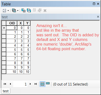
Lets start with a small point data file brought in from Arcmap using the FeatureClassToNumPyArray tool.

Four fields were brought in, the Shape field ( as X and Y values), an integer Group field and a Text field.  The data types for each field are indicated in the dtype line.   The details of data types have been documented in other documents in the series.

>>> arr
array([(6.0, 0.0, 4, 'a'), (7.0, 9.0, 2, 'c'),
       (8.0, 6.0, 1, 'b'), (3.0, 2.0, 4, 'a'),
       (6.0, 0.0, 4, 'a'), (2.0, 5.0, 2, 'b'),
       (3.0, 2.0, 4, 'a'), (8.0, 6.0, 1, 'b'),
       (7.0, 9.0, 2, 'c'), (6.0, 0.0, 4, 'a')],
      dtype=[('X', '<f8'), ('Y', '<f8'), ('Group', '<i4'), ('Text', 'S5')])
>>> arr.shape
(10,)
‍‍‍‍‍‍‍‍‍

In summary:

  • the X and Y fields 64 bit floating point numbers (denoted by: <f8 or  float64)
  • the Group field is a 32 bit integer field (denoted by: <i4 or int32)
  • the text field is just that...a field of string data 5 characters wide.

Is any of this important?  Well yes...look at the array above. The shape indicates it has 10 rows but no columns??  Not quite what you were expecting and it appears all jumbled and not nicely organized like a table in ArcMap or in a spreadsheet.  The array is a structured array, a subclass of the multidimensional array class, the  ndarray.  The data types in structured arrays are mixed and NumPy works if the data are of one data type like those in the parent class

Data in an array can be cast to find a common type, if it contains one element belongs to a higher data type.  Consider the following examples, which exemplify this phenomenon.

The arrays have been cast into a data type which is possible for all elements.  For example, the 2nd array contained a single floating point number and 4 integers and upcasting to floating point is possible.  The 3rd example downcast the integers to string and in the 4th example, True was upcast to integer since it has a base class of integer, which is why True-False is often represented by 1-0.

>>> type(True).__base__
<type 'int'>
‍‍

The following code will be used for further discussion.

def get_unique(arr,by_flds=[]):
    """ Produce unique records in an array controlled by a list of fields.
    Input:   An array, and a list of fields to assess unique.
        All fields:  Use [] for all fields. 
        Remove one:  all_flds = list(arr_0.dtype.names)
                     all_flds.remove('ID')
        Some fields: by name(s): arr[['X','Y']]  # notice the list inside the slice
                     or slices:  all_flds[slice]... [:2], [2:], [:-2] [([start:stop:step])
    Returns: Unique array of sorted conditions.
             The indices where a unique condition is first encountered.
             The original array sliced with the sorted indices.
    Duh's:   Do not forget to exclude an index field or fields where all values are
             unique thereby ensuring each record will be unique and you will fail miserably.
    """
    a = arr.view(np.recarray)
    if by_flds:
        a = a[by_flds].copy()
    N = arr.shape[0]
    if arr.ndim == 1: # ergo... arr.size == arr.shape[0]
        uniq,idx = np.unique(a,return_index=True)
        uniq = uniq.view(arr.dtype).reshape(-1, 1) # purely for print purposes
    else:
        uniq,idx = np.unique(arr.view(a.dtype.descr * arr.shape[1]),return_index=True)
        uniq = uniq.view(arr.dtype).reshape(-1, arr.shape[1])
    arr_u = arr[np.sort(idx)]
    return uniq,idx,arr_u

if __name__=="__main__":
    """Sample data section and runs...see headers"""
    X = [6,7,8,3,6,8,3,2,7,9];  Y = [0,9,6,2,0,6,2,5,9,4]
    G = [4,2,1,4,3,2,2,3,4,1];  T = ['a','c','b','a','a','b','a','c','d','b']
    dt = [('X','f8'),('Y','f8'),('Group','i4'),('Text','|S5')]
    arr_0 = np.array(zip(X,Y,G,T),dtype=dt)
    uniq_0,idx_0,arr_u0 = get_unique(arr_0[['X','Y']])
    frmt = "\narr_0[['X','Y']]...\nInput:\n{}\nOutput:\n{}\nIndices\n{}\nSliced:\n{}"
    print(frmt.format(arr_0,uniq_0,idx_0,arr_u0))

‍‍‍‍‍‍‍‍‍‍‍‍‍‍‍‍‍‍‍‍‍‍‍‍‍‍‍‍‍‍‍‍‍‍‍‍‍

Which yields the following results

arr_0[['X','Y']]...
Input:
[(6.0, 0.0, 4, 'a') (7.0, 9.0, 2, 'c') (8.0, 6.0, 1, 'b')
 (3.0, 2.0, 4, 'a') (6.0, 0.0, 3, 'a') (8.0, 6.0, 2, 'b')
 (3.0, 2.0, 2, 'a') (2.0, 5.0, 3, 'c') (7.0, 9.0, 4, 'd')
 (9.0, 4.0, 1, 'b')]
Output:
[[(2.0, 5.0)]
 [(3.0, 2.0)]
 [(6.0, 0.0)]
 [(7.0, 9.0)]
 [(8.0, 6.0)]
 [(9.0, 4.0)]]
Indices
[7 3 0 1 2 9]
Sliced:
[(6.0, 0.0) (7.0, 9.0) (8.0, 6.0) (3.0, 2.0) (2.0, 5.0)
 (9.0, 4.0)]
‍‍‍‍‍‍‍‍‍‍‍‍‍‍‍‍‍‍

The arr_0 output is your conventional recarray output with everything wrapped around making it hard to read.  The Output section showsn the unique X,Y values in the array in sorted order, which is the default.  The Indices output is the location in the original array where the entries in the sorted Output can be found.  To produce the Sliced incarnation, I sorted the Indices, then used the sorted indices to slice the rows out of the original array.

Voila...take a table, make it an array...find all the unique entries based upon the whole array, or a column or columns, then slice and dice to get your desired output.  In any event, it is possible to terminate the process at any point and just find the unique values in a column for instance.

The next case will show how to deal with ndarrays which consist of a uniform data type and the above example will not work.

Of course there is a workaround.  To that end, consider the small def from a series I maintain, that shows how to recast an ndarray with a single dtype to a named structured array and a recarray.  Once you have fiddled with the parts, you can 

  • determine the unique records (aka rows)
  • get them in sorted order or
  • maintain the original order of the data

# ----------------------------------------------------------------------
# num_42 comment line above def
def num_42():
    """(num_42)...unique while maintaining order from the original array
    :Requires: import numpy as np
    :--------
    :Notes:  see my blog for format posts, there are several
    :-----
    : format tips
    : simple  ["f{}".format(i) for i in range(2)]
    :         ['f0', 'f1']
    : padded  ["a{:0>{}}".format(i,3) for i in range(5)]
    :         ['a000', 'a001', 'a002', 'a003', 'a004']
    """
    a = np.array([[2, 0], [1, 0], [0, 1], [1, 0], [1, 2], [1, 2]])
    shp = a.shape
    dt_name = a.dtype.name
    flds = ["f{:0>{}}".format(i,2) for i in range(shp[1])]
    dt = [(fld, dt_name) for fld in flds]
    b = a.view(dtype=dt).squeeze()  # type=np.recarray,
    c, idx = np.unique(b, return_index=True)
    d = b[idx]
    return a, b, c, idx, d‍‍‍‍‍‍‍‍‍‍‍‍‍‍‍‍‍‍‍‍‍‍‍

The results are pretty well as expected.  

  1. Array 'a' has a uniform dtype.
  2. The shape and dtype name were used to produce a set of field names (see flds and dt construction).
  3. Once the dtype was constructed, a structured or recarray can be created ( 'b' as structured  array).
  4. The unique values in array 'b' are returned in sorted order ( array 'c', see line 21)
  5. The indices of the first occurrence of the unique values are also returned (indices, idx, see line 21)
  6. The input structured array, 'b', was then sliced using the indices obtained.
>>> a
array([[2, 0],
       [1, 0],
       [0, 1],
       [1, 0],
       [1, 2],
       [1, 2]])
>>> b
array([(2, 0), (1, 0), (0, 1), (1, 0), (1, 2), (1, 2)], 
      dtype=[('f00', '<i8'), ('f01', '<i8')])
>>> c
array([(0, 1), (1, 0), (1, 2), (2, 0)], 
      dtype=[('f00', '<i8'), ('f01', '<i8')])
>>> idx
array([2, 1, 4, 0])
>>> d
array([(0, 1), (1, 0), (1, 2), (2, 0)], 
      dtype=[('f00', '<i8'), ('f01', '<i8')])‍‍‍‍‍‍‍‍‍‍‍‍‍‍‍‍‍‍‍‍‍‍‍‍‍‍‍‍‍‍‍‍‍‍‍‍
>>> # or via original order.... just sort the indices
>>> idx_2 = np.sort(idx)
>>> idx_2
array([0, 1, 2, 4])
>>> b[idx_2]
array([(2, 0), (1, 0), (0, 1), (1, 2)], 
      dtype=[('f00', '<i8'), ('f01', '<i8')])

I am sure a few of you (ok, maybe one), is saying 'but the original array was a Nx2 array with a uniform dtype?  Well I will leave the solution for you to ponder.  Once you understand it, you will see that it isn't that difficult and you only need  a few bits of information... the original array 'a' dtype, and shape and the unique array's shape...

>>> e = d.view(dtype=a.dtype).reshape(d.shape[0],a.shape[1])
>>> e
array([[0, 1],
       [1, 0],
       [1, 2],
       [2, 0]])‍‍‍‍‍‍

These simple examples can be upcaled quite a bit in terms of the number of row and columns and which ones you need to participate in the uniqueness quest.

That's all for now.  

more
2 2 3,534
DanPatterson_Retired
MVP Emeritus

Numpy_Snippets

Updated: 2016-09-09

Previous snippets:

None                   Jan 5, 2015

Documentation   Jan 30

Edits                    May 5

Documentation

NumPy Reference — NumPy v1.9 Manual

Tentative NumPy Tutorial -

for numpy python packages

http://www.lfd.uci.edu/~gohlke/pythonlibs/

other links

http://rintintin.colorado.edu/~wajo8931/docs/jochem_aag2011.pdf

-------------------------------------------------------------------------------------------------

As a companion to the Numpy Lessons series, I have posted within my blog, I have decided to maintain a series of snippets that don't comfortably fit into a coherent lesson.  They, like the lessons, will be sequentially numbered with links to the previous ones kept in the top section.  Contributions and/or corrections.

All samples assume that the following imports are made.  Other required imports will be noted when necessary.

# default imports used in all examples whether they are or not
import numpy as np
import arcpy
‍‍‍

This is a bit of a hodge-podge, but the end result is produce running means for a data set over a 10-year time period.
Simple array creation is shown using two methods, as well as how to convert array contents to specific data types.

>>> year_data = np.arange(2005,2015,dtype='int')   # 10 years worth of records from 2005 up to, but not 2015
>>> some_data = np.arange(0,10,dtype='float')      # some numbers...sequential and floating point in this case
>>> result = np.zeros(shape=(10,),dtype='float')   # create an array of 0's with 10 records
>>> result.fill(-999)                              # provide a null value and fill the zero's with null values
>>> result_list = zip(year_data,some_data,result)  # zip the 3 arrays together
>>> 
>>> dt = np.dtype([('year','int'), ('Some_Data', 'float'),('Mean_5year',np.float64)]) # combined array type
>>> result_array = np.array(result_list,dtype=dt)  # produce the final array with the desired data type
>>> result_array
array([(2005, 0.0, -999.0), (2006, 1.0, -999.0), (2007, 2.0, -999.0),
       (2008, 3.0, -999.0), (2009, 4.0, -999.0), (2010, 5.0, -999.0),
       (2011, 6.0, -999.0), (2012, 7.0, -999.0), (2013, 8.0, -999.0),
       (2014, 9.0, -999.0)], 
      dtype=[('year', '<i4'), ('Some_Data', '<f8'), ('Mean_5year', '<f8')])
>>>
‍‍‍‍‍‍‍‍‍‍‍‍‍‍‍

The result_array now consists of a three columns, which can be accessed by names using array slicing.

>>> result_array['year']                           # slicing the year, data and result column values
array([2005, 2006, 2007, 2008, 2009, 2010, 2011, 2012, 2013, 2014])
>>> result_array['Some_Data']
array([ 0.,  1.,  2.,  3.,  4.,  5.,  6.,  7.,  8.,  9.])
>>> result_array['Mean_5year']
array([-999., -999., -999., -999., -999., -999., -999., -999., -999., -999.])
>>>
‍‍‍‍‍‍‍

If this array, an ndarray, is converted to a recarray, field access can also be achieved using 'array.field' notation.

>>> result_v2 = (result_array.view(np.recarray))   # convert it to a recarray to permit 'array.field access'
>>> 
>>> result_v2.year
array([2005, 2006, 2007, 2008, 2009, 2010, 2011, 2012, 2013, 2014])
>>> result_v2.Some_Data
array([ 0.,  1.,  2.,  3.,  4.,  5.,  6.,  7.,  8.,  9.])
>>> result_v2.Mean_5year
array([-999., -999., -999., -999., -999., -999., -999., -999., -999., -999.])
>>>
‍‍‍‍‍‍‍‍‍

The remainder of the demonstration basically shows some of the things that can be done with ndarrays and recarrays.  As an example, the 5-year running mean will be calculated and the Mean_5year column's null values replaced with valid data.  The 'np.convolve' method will be used to determine the running means for no other reason than I hadn't used it before.  Since the input data are sequential numbers from 0 to 9, it will be pretty easy to do the mental math to figure out whether the running mean is indeed correct.  The steps entail:

  1. decide upon the mean step to use (eg. N=5),
  2. run the convolve method on the 'Some_Data' column in the result_v2 recarray,
  3. pad the resultant array so that the sizes of the running mean calculation array and the column array are equal.

Here it goes...

>>> N = 5                                          # five year running mean step, see the help on convolve
>>> rm = np.convolve(result_v2['Some_Data'],np.ones((N,))/N, mode='valid')  # a mouth-full
>>> rm                                             # however, there are only values for the mid-point year
array([ 2.,  3.,  4.,  5.,  6.,  7.])              # so we need to pad by 2 on either end of the output
>>> 
>>> pad_by = N/2                                   # integer division...this has change in python 3.x
>>>
>>> new_vals = np.pad(rm,pad_by,mode='constant',constant_values=-999)   # padding the result to new_vals
>>> new_vals
array([-999., -999.,    2.,    3.,    4.,    5.,    6.,    7., -999., -999.])
>>>
>>> result_v2.Mean_5year = new_vals                # set the new_vals into the correct column
>>> 
>>> result_v2                                      # voila
rec.array([(2005, 0.0, -999.0), (2006, 1.0, -999.0), (2007, 2.0, 2.0),
       (2008, 3.0, 3.0), (2009, 4.0, 4.0), (2010, 5.0, 5.000000000000001),
       (2011, 6.0, 6.0), (2012, 7.0, 7.000000000000001),
       (2013, 8.0, -999.0), (2014, 9.0, -999.0)], 
      dtype=[('year', '<i4'), ('Some_Data', '<f8'), ('Mean_5year', '<f8')])
>>> 
‍‍‍‍‍‍‍‍‍‍‍‍‍‍‍‍‍‍‍‍


A bit messy with that floating point representation thing appearing for a few numbers....let's clean it up by changing the dtype to limit the number of decimal points in the array showing up in the 'Mean_5year column.  This will be done incrementally.

>>> x = np.round(result_v2.Mean_5year,decimals=2)
>>> result_v2.Mean_5year = x
>>> result_v2
rec.array([(2005, 0.0, -999.0), (2006, 1.0, -999.0), (2007, 2.0, 2.0),
       (2008, 3.0, 3.0), (2009, 4.0, 4.0), (2010, 5.0, 5.0),
       (2011, 6.0, 6.0), (2012, 7.0, 7.0), (2013, 8.0, -999.0),
       (2014, 9.0, -999.0)], 
      dtype=[('year', '<i4'), ('Some_Data', '<f8'), ('Mean_5year', '<f8')])
>>>
‍‍‍‍‍‍‍‍‍

So these snippets have shown some of the things that can be done with arrays and the subtle but important distinctions between numpy's array, ndarray and recarray forms.

more
2 0 1,861
DanPatterson_Retired
MVP Emeritus

Numpy Snippets

Updates: 2016-09-09

This just a quick example of how to use existing arrays and export them to tables.  In this case I will use arcpy functionality to produce a dBase file.  Numpy can be used directly to produce text files as well.

To begin with:

  • two arrays of X and Y values are created in the range 0-10 inclusive (ie 11 numbers),
  • a data type is specified (dt)... in this case I assigned 'X' and 'Y' to the columns and specified a 64-bit floating point number,
  • an array, XY, is create using some fancy zipping of the original arrays with the specified data type,
  • ArcPy is imported, an output table is created using the data access module's NumPyArrayToTable.
  • Now for the magical reveal

>>> import numpy as np
>>> X = np.arange(11)                # take some numbers
>>> Y = np.arange(11)                # ditto
>>> dt = [('X','<f8'),('Y','<f8')]   # specify a data type ie 64 bit floats
>>> 
>>> XY = np.array(zip(X,Y), dtype = dt) # create a 2D array of floats
>>> XY
array([(0.0, 0.0), (1.0, 1.0), (2.0, 2.0), (3.0, 3.0), (4.0, 4.0),
       (5.0, 5.0), (6.0, 6.0), (7.0, 7.0), (8.0, 8.0), (9.0, 9.0),
       (10.0, 10.0)], 
      dtype=[('X', '<f8'), ('Y', '<f8')])
>>> 
>>> import arcpy                     # now lets do some arcpy stuff
>>> out_table = 'c:/temp/test.dbf'
>>> arcpy.da.NumPyArrayToTable(XY,out_table)
‍‍‍‍‍‍‍‍‍‍‍‍‍‍‍‍‍‍‍‍‍‍‍‍‍‍‍‍‍‍‍‍‍‍‍‍‍‍‍‍‍‍‍‍‍‍‍‍‍‍‍‍‍‍‍‍‍‍‍‍‍‍‍‍‍‍‍‍‍‍‍‍‍‍‍‍‍‍‍

: -----------------------------------------------------

Now for the reveal...

Output_Table.jpg

: -----------------------------------------------------

Bring it back you say?   Nothing could be easier.

>>> in_array = arcpy.da.TableToNumPyArray(out_table,['OID','X','Y'])
>>> in_array
array([(0, 0.0, 0.0), (1, 1.0, 1.0), (2, 2.0, 2.0), (3, 3.0, 3.0),
       (4, 4.0, 4.0), (5, 5.0, 5.0), (6, 6.0, 6.0), (7, 7.0, 7.0),
       (8, 8.0, 8.0), (9, 9.0, 9.0), (10, 10.0, 10.0)], 
      dtype=[('OID', '<i4'), ('X', '<f8'), ('Y', '<f8')])
‍‍‍‍‍‍‍‍‍‍‍‍‍‍‍‍‍‍‍‍‍‍‍‍‍‍‍‍‍‍‍‍‍‍‍‍‍‍‍‍‍‍‍‍‍‍‍‍‍

: -----------------------------------------------------

Out to *.csv you say?  Too easy (nothing fancy this time...just the numbers but formatted a bit).

    0,      0.00,      0.00
    1,      1.00,      1.00
    2,      2.00,      2.00
    3,      3.00,      3.00
    4,      4.00,      4.00
    5,      5.00,      5.00
    6,      6.00,      6.00
    7,      7.00,      7.00
    8,      8.00,      8.00
    9,      9.00,      9.00
   10,     10.00,     10.00
‍‍‍‍‍‍‍‍‍‍‍‍‍‍‍‍‍‍‍‍‍‍‍‍‍‍‍‍‍‍‍‍‍‍‍‍‍‍‍‍‍‍‍‍‍‍‍‍‍‍‍‍‍‍‍‍‍‍‍

So NumPy and ArcPy do play 'nice' together.  Experiment a bit.   More later.

more
1 0 2,121
DanPatterson_Retired
MVP Emeritus

Numpy Snippets

Updated: 2016-09-09

The purpose of this post is to show how numpy can play nicely with arcpy to produce geometry and perform tasks like shape translation, rotation and scaling which are not readily available in arcpy's available functions.

To pay homage to ArcMap's ... Fish Net ... I propose a very scaled down version aptly named Phish_Nyet.  A fuller version will appear when ArcScript 2.0 opens.  This is a demo script.  All you do is vary the parameters in the demo() function within the script.

Sampling_grids.png

Only the rectangular option will be presented here, however, it is possible to make all kinds of sampling grids, including hexagonal ones as shown above.

The following points apply:

  • Output is to a shapefile.
  • The output file must have a projected coordinate system.   To create grids in Geographic coordinates, use Fishnet in ArcMap.  Why?  because invariably people create grids in Geographic coordinates, then project them without densifying the grid blocks.  This results in shapes which are in error because the curvature associated with lines of latitude are not accounted for.
  • A corner point is specified as the origin of the net.  One can determine which corner to use by specifying a dX and dY with positive and/or negative values.  In this fashion, you can get your corner to be the top or bottom, left or right of the output.  If you want the middle to be the origin...do the math and get a corner.
  • The output is controlled by the cell widths (dX and dY), the number of columns and rows an (i.e.  the X and Y directions) and a rotation angle, which is positive for clockwise rotation.

Notes:

  - grid_array - does the numpy magic of generating the grid shapes.   I have tried to be as verbose as possible.  In short, I generate a

    seed shape and propagate it.  I have intentionally kept rotate and  output_polygons as visible function so you can see how they work.

A fuller version will surface as I stated when ArcScripts 2.0 appears.  Change the parameters in the demo() function and run it.

"""
Phish_Nyet.py
Author:  Dan.Patterson@carleton.ca

Purpose: Produce a sampling grid with user defined parameters.
"""
import arcpy
import numpy as np

def demo():
    """Generate the grid using the following parameter"""
    output_shp = r'C:\temp\Phish_Nyet.shp'
    SR =  arcpy.SpatialReference(2951) # u'NAD_1983_CSRS_MTM_9' YOU NEED ONE!!!
    corner = [340000.0, 5022000.0]     # corner of grid 
    dX = 1000.0;  dY = 1000.0          # X and Y cell widths
    cols = 3;  rows = 3                # columns/rows...grids in X and Y direction
    angle = 0                          # rotation angle, clockwise +ve
    # create the grid 
    pnts = grid_array(corner,dX,dY,cols,rows,angle)
    output_polygons(output_shp,SR,pnts)
    print('\nPhish_Nyet has created... {}'.format(output_shp))

def grid_array(corner=[0,0],dX=1,dY=1,cols=1,rows=1,angle=0):
    """create the array of pnts to pass on to arcpy using numpy magic"""
    X = [0.0,0.0,1.0,1.0,0.0]                  # X,Y values for a unit square
    Y = [0.0,1.0,1.0,0.0,0.0]                  # 
    seed = np.column_stack((X,Y)) * [dX,dY]    # first array corner values scaled
    u = [seed + [j*dX,i*dY] for i in range(0,rows) for j in range(0,cols)]
    pnts = np.array(u)                         # 
    x = [rotate(p,angle) for p in pnts]        # rotate the scaled points 
    pnts = [ p + corner for p in x]            # translate them
    return pnts

def rotate(pnts,angle=0):
    """rotate points about the origin in degrees, (+ve for clockwise) """
    angle = np.deg2rad(angle)               # convert to radians
    s = np.sin(angle);  c = np.cos(angle)   # rotation terms
    aff_matrix = np.array([[c, -s],[s, c]]) # rotation matrix
    XY_r = np.dot(pnts, aff_matrix)         # numpy magic to rotate pnts
    return XY_r

def output_polygons(output_shp,SR,pnts):
    """produce the output polygon shapefile"""
    msg = '\nRead the script header... A projected coordinate system required'
    assert (SR != None) and (SR.type=='Projected'), msg
    polygons = []
    for pnt in pnts:                           # create the polygon geometry
        polygons.append(arcpy.Polygon(arcpy.Array([arcpy.Point(*xy) for xy in pnt]),SR))
    if arcpy.Exists(output_shp):               # overwrite any existing versions
        arcpy.Delete_management(output_shp)
    arcpy.CopyFeatures_management(polygons, output_shp)

if __name__ == '__main__':
    """Generate the grid using the listed parameters"""
    demo()  # modify the parameters in demo to run
‍‍‍‍‍‍‍‍‍‍‍‍‍‍‍‍‍‍‍‍‍‍‍‍‍‍‍‍‍‍‍‍‍‍‍‍‍‍‍‍‍‍‍‍‍‍‍‍‍‍‍‍‍‍‍‍‍‍‍‍‍‍‍‍‍‍‍‍‍‍‍‍‍‍‍‍‍‍‍‍‍‍‍‍‍‍‍‍‍‍‍‍‍‍‍‍‍‍‍‍‍‍‍‍‍‍‍‍‍‍‍‍‍‍‍‍‍‍‍‍‍‍‍‍‍‍‍‍‍‍‍‍‍‍‍‍‍‍‍‍‍‍‍‍‍‍‍‍‍‍‍‍‍‍‍‍‍‍‍‍‍‍‍‍

Of course other regular geometric shapes can be generated in a similar fashion, but not all may pack like rectangles and others do.

more
4 11 4,790
DanPatterson_Retired
MVP Emeritus

N-gon Demo

Updated:  2018-08-24  Added Triangles and a better labelling system

Created a toolbox and script tool for ArcGIS PRO 2.2 on the Code Sharing site... Sampling Grid ....

Yes... 'Pointy' and 'Flat Head' now have a home as well as rectangular sampling grids.  I also added cell labelling, akin to how spreadsheet cells are labelled (A1, B1 etc)

: -------------

The Toolbox

Your inputs are simple

For those interested in parameter setup for tools

: -------------

This post .... how to draw octagon or hexagon in ArcGIS desktop ?  lead me back to an original post dealing with producing sampling grids.Numpy Snippets # 3 ... Phish_Nyet ... creating sampling grids using numpy and arcpy   For completeness, here are further thoughts.

There are two implementations of n-gons...flat topped and pointy topped.  They only differ by the rotation angle relative to the X/Y axis.  In the case of a square, the rotation is 45°. And yes...even a circle in ArcMap is represented as a 360-sided n-gon so it does have a pointy and a flat top.

Once the seed shape is created, it can be placed around the centroid of known points by creating a polygon from the array outputs.  I normally use FeatureclassToNumPyArray and NumPyArrayToFeatureclass to perform the transition from points to array and back again.  In my previous blog, I exploited this to produce a sampling grid using rectangles and hexagons of know width, location and orientation for both the flat and pointy topped examples.

There is nothing stopping one from creating any geometric shape in any configuration using these simple principles.  All that needs to be determined is the angles needed to produce the n-gon.  For example, the only two lines that need to be changed are these to represent the polygon (n-gon) angles.  From there, the desired width is used to create the final seed which can then be shifted into the desired configuration/location using other code samples included in my previous blogs.

Flat topped f_rad = np.deg2rad([180.,120.,60.,0.,-60.,-120.,-180.])        angles in degrees

Point topped p_rad = np.deg2rad([150.,90,30.,-30.,-90.,-150.,150.])

See the script with the toolbox on the download site for more complete code samples.

"""
hexagon_demo_shape.py
Author:  
Dan.Patterson@carleton.ca

Purpose: create hexagon shapes in two forms, flat-topped and pointy-topped
Result:
   Produce hexagon of desired width in X direction centered about
   the origin (0,0)
NOTES:   see full code for other implementations
"""
import numpy as np
np.set_printoptions(precision=4,threshold=10,edgeitems=5,linewidth=75,suppress=True)
def hex_flat(size=1,cols=1,rows=1):
    """generate the points for the flat-headed hexagon """
    f_rad = np.deg2rad([180.,120.,60.,0.,-60.,-120.,-180.])
    X = np.cos(f_rad)*size;  Y = np.sin(f_rad)*size # scaled hexagon about 0,0
    seed = np.array(zip(X,Y))            # array of coordinates
    return seed

def hex_pointy(size=1,cols=1,rows=1):
    """pointy hex angles, convert to sin,cos, zip and send"""
    p_rad = np.deg2rad([150.,90,30.,-30.,-90.,-150.,150.]) 
    X = np.cos(p_rad)*size;  Y = np.sin(p_rad)*size # scaled hexagon about 0,0
    seed = np.array(zip(X,Y))
    return seed

if __name__ == '__main__':
    flat = hex_flat(700,1,1)
    pointy = hex_pointy(700,1,1)
    print('\nFlat headed hexagon \n{}'.format(flat))
    print('\nPointy headed hexagon \n{}'.format(pointy))
‍‍‍‍‍‍‍‍‍‍‍‍‍‍‍‍‍‍‍‍‍‍‍‍‍‍‍‍‍‍‍‍‍‍‍‍‍‍‍‍‍‍‍‍‍‍‍‍‍‍‍‍‍‍‍‍‍‍‍‍‍‍‍‍‍‍‍‍‍‍‍‍‍‍‍‍‍‍‍‍‍‍‍‍‍‍‍‍‍‍‍‍‍‍‍‍‍‍‍‍‍‍‍‍‍‍‍‍‍‍‍‍‍‍‍‍‍‍‍‍‍‍‍‍‍‍‍‍‍‍‍‍‍‍‍‍‍‍‍‍‍‍‍‍‍‍‍‍‍‍‍‍‍‍‍‍‍‍‍‍‍‍‍‍‍‍‍‍‍‍‍‍‍‍‍‍‍‍‍‍‍‍‍‍‍‍‍‍‍‍‍‍‍‍‍‍‍

Outputs for flat and pointy headed hexagons.

1 m width (unit width)100 Unit width700 m width

Flat headed hexagon

[[-1.     0.   ]

[-0.5    0.866]

[ 0.5    0.866]

[ 1.     0.   ]

[ 0.5   -0.866]

[-0.5   -0.866]

[-1.    -0.   ]]

Flat headed hexagon

[[-100.        0.    ]

[ -50.       86.6025]

[  50.       86.6025]

[ 100.        0.    ]

[  50.      -86.6025]

[ -50.      -86.6025]

[-100.       -0.    ]]

Flat headed hexagon

[[-700.        0.    ]

[-350.      606.2178]

[ 350.      606.2178]

[ 700.        0.    ]

[ 350.     -606.2178]

[-350.     -606.2178]

[-700.       -0.    ]]

Flat headed hexagon

[[-1.     0.   ]

[-0.5    0.866]

[ 0.5    0.866]

[ 1.     0.   ]

[ 0.5   -0.866]

[-0.5   -0.866]

[-1.    -0.   ]]

Pointy headed hexagon

[[ -86.6025   50.    ]

[   0.      100.    ]

[  86.6025   50.    ]

[  86.6025  -50.    ]

[   0.     -100.    ]

[ -86.6025  -50.    ]

[ -86.6025   50.    ]]

Pointy headed hexagon

[[-606.2178  350.    ]

[   0.      700.    ]

[ 606.2178  350.    ]

[ 606.2178 -350.    ]

[   0.     -700.    ]

[-606.2178 -350.    ]

[-606.2178  350.    ]]

Enjoy.  Should one require the rotation code or shape generation code, let me know or check the code for guidance in NumPy Snippets # 3

more
5 4 3,493
229 Subscribers
Labels