Use the Five-Step GIS Analysis Process

Suzanne-Boden · ‎10-19-2018

This post shows how to apply a five-step process to complete an analysis project using ArcMap (the same analysis could be performed just as easily in ArcGIS Pro). Suppose you want to analyze access to health care services in Riverside and San Bernardino counties in southern California.

The five steps in the analysis process are:

Frame the question
Explore and prepare data
Choose analysis methods and tools
Perform the analysis
Examine and refine results

Step 1. Frame the Question
This step seems straightforward because typically you're assigned a project to obtain specific information. Some projects involve answering several questions derived from a high-level question. How you frame the questions helps determine which GIS tools and methods you use for the analysis.

In this example, you might frame a preliminary high-level question: Is the distribution of health care facilities consistent with the population distribution in Riverside-San Bernardino, CA? This question could be broken down into the following sub-questions:

Where are facilities that provide health care services located?
What is the population distribution within the study area?
Do areas with the highest population density have the greatest number of facilities?
Within the study area, are there areas with high population density but no health care facilities?

Step 2. Explore and Prepare Data
This step can be the most time-consuming. If you don't have all the data needed for an analysis project, you must collect it. The ArcGIS Living Atlas of the World is an excellent source of high-quality spatial data. In the U.S., the Census Bureau has a multitude of spatial, population, and demographic data. State data clearinghouses are another useful resource.

Step 2a: Explore Data
For each dataset, explore the feature geography, attributes, and metadata to determine whether the data will be useful for your analysis and what kind of preparation, if any, may be required. Questions to ask about the data include:

What is the data format?
When was the data collected (how current is it)?
How detailed is the data—at what scale was it collected?
What coordinate system does the data use? Is the data projected?
- Best practice is to project all datasets into a common coordinate system before doing analysis.
Does the feature geometry (i.e., point, line, polygon) work for the analysis?
Does the data have the attributes you need?
Does the data have any access or use constraints?

For this example, the following datasets were used. All use the WGS 1984 geographic coordinate system.

Hospitals — this data includes "traditional" hospitals as well as other medical facilities.
ZIP Codes — this data includes population attributes.
Counties — this data provides the geography for the area of interest (Riverside and San Bernardino counties).
States — this data provides additional geographic reference for the area of interest (California).

Step 2b: Prepare Data
To start, you need to decide what data format to use. Project data doesn't have to be all in the same format, but it can make things easier. The important thing is to verify that the analysis tools you need to use accept your data format; also consider whether you will be distributing the data created by the analysis. You can use the geoprocessing tools in the ArcToolbox Conversion Tools toolbox to quickly convert data to another format. If you have access to the ArcGIS Data Interoperability extension, you can directly work with many data formats.

Organizing data into a project folder helps simplify analysis tasks (you can specify a default input workspace for all the geoprocessing tools).

For this project, a file folder was created to organize the shapefiles.

If you are working with feature classes stored in different geodatabases, you could copy or import them into a single file-based project geodatabase. You might also want to create separate folders or geodatabases to store intermediate (temporary) data output from analysis operations as well as final data.

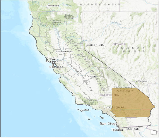
Extracting data to have the same extent as the study area helps speed up processing time and enhances data visualization in ArcMap. In this example, the project datasets cover the entire U.S.

Clipping the hospitals and ZIP Codes to the extent of the two counties will be part of data preparation.

In order to clip the data, you can create a selection layer of just Riverside and San Bernardino counties, or just select the two counties on the map. If you plan to use the same study area for multiple analysis projects, it's a good idea to export selected features and selection layers to their own shapefile or geodatabase feature class. That way, you have your study area feature data ready to go. For this example, we will simply select the two counties of interest.

Here's are the data preparation tasks for this project:

Start ArcMap, add the project data, and zoom to the study area.
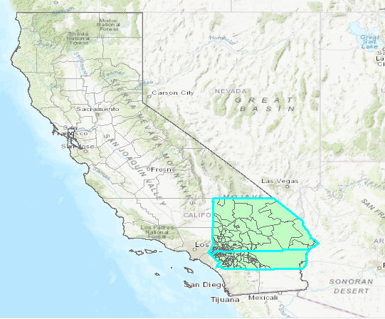
Using the Select Features tool, select Riverside and San Bernardino counties. Now you will clip the U.S. ZIP Codes to the extent of the two counties.
Open ArcToolbox, expand Analysis Tools, expand Extract, and double-click Clip to open the tool dialog box.
For Input Features, choose U.S. ZIP Codes. For Clip Features, choose Counties. When the clip layer has selected features, only the selected features will be used to clip the input features.
Accept or change the output location and name, then click OK to run the tool.
The clipped layer that contains only ZIP Codes in Riverside and San Bernardino counties is added to the Table of Contents.

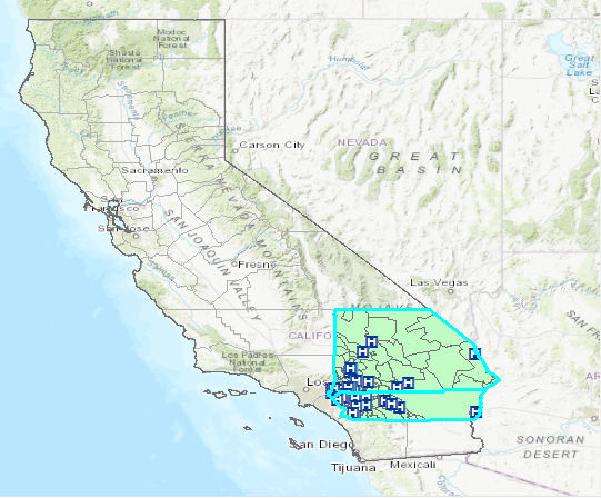
Repeat the steps to clip the hospitals.

Double-click the Clip tool to open its dialog box.
For Input Features, choose Hospitals.
For Clip Features, choose Counties.
For Output Feature Class, accept or change the default output location and name, then click OK.

When the clip operation completes, a layer representing hospitals within the study area is added to the Table of Contents.

Change the default symbol as desired and remove the U.S. hospitals and ZIP Code layers (right-click each layer in the Table of Contents and choose Remove).

The data preparation tasks are now complete.

Step 3. Choose Analysis Methods and Tools

To choose the appropriate methods and tools for an analysis project, consider the questions framed in step 1 and document the methods and tools that will answer each one.

Question	Methods and Tools
Where are facilities that provide health care services located?	Examine distribution of hospitals on the map.
What is the population distribution within the study area?	Symbolize ZIP Codes layer based on population density using graduated colors.
Do areas with the highest population density have the greatest number of facilities?	First, do a visual analysis of the map to get a general idea, then do a spatial join operation between the Hospitals and ZIP Codes. The output of the spatial join will be one record for each hospital and the ZIP Code attributes.
Within the study area, are there areas with high population but no health care facilities?	Summarize the ZIP field in the table output from the spatial join. The summary table will include a count of hospitals in each ZIP code that contains a hospital, plus population data for each ZIP Code.

It's helpful at this step to diagram the analysis. The diagram doesn't have to be anything fancy (although it can be if you like that sort of thing). An easy thing is to quickly draw on paper or a whiteboard like the example below.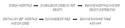

Step 4. Perform the Analysis
If you've diagrammed the process in step 3, then in this step, you simply follow the diagram, completing each task in sequence. For complicated analyses, you may want to create a model in ModelBuilder to automate the process. A model also allows you to quickly change a parameter and run the model again to explore different scenarios.

Examine the distribution of the hospital features on the map. Zoom and pan around as needed.
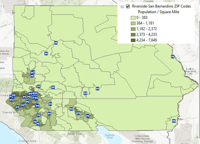
Symbolize ZIP Codes with graduated colors based on the POP07_SQMI (2007 population density) attribute.

A visual analysis of the data shows the greatest number of hospitals and the most densely populated ZIP Codes (in darker shades of green on the map below) are in the southwestern part of the study area.

You can get more information by doing a spatial join between the Hospitals and ZIP Codes layers.

Right-click Hospitals and click Joins and Relates > Join.
In the dialog box, choose to join data from another layer based on spatial location.
Choose ZIP Codes in the drop-down list of layers, specify the output feature class name and location, and click OK.

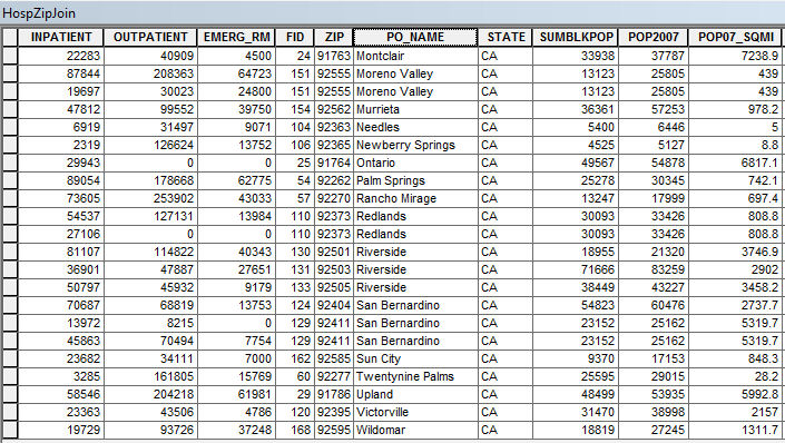
The output of the spatial join is a new point layer that contains all the hospital features plus the attributes of the ZIP Code each facility falls within. The ZIP field contains the five-digit ZIP Code in which the hospital is located, and the PO_NAME field contains the post office name (corresponds to the city name) for that ZIP Code. The POP07_SQMI field shows the population density associated with each hospital's ZIP Code.

Sorting the PO_NAME field reveals that multiple hospitals are located in some ZIP Codes.

The last step is to summarize the ZIP field. This operation will output a table that contains one record for each ZIP Code that contains a hospital, plus a field containing the count of hospitals within each ZIP Code. You can also choose to output statistics for numeric fields (such as POP07_SQMI).

In the joined table, right-click the ZIP field and choose Summarize.
For summary statistics, check First and Last for NAME (this is the hospital name) and check Average for both POP2007 (total population) and POP07_SQMI.
Specify an output location and name, then click OK.
Choose to add the result table to the map and open it.

Step 5. Examine and Refine Results

So what information does the summary table provide?

The Count_ZIP field tells you the number of hospitals in each ZIP Code that contains a hospital.

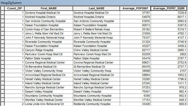
Sorting the POP07_SQMI field reveals that all the ZIP Codes that have more than 2,000 people per square mile have at least one health care facility.

The analysis shows that the distribution of health care services is generally consistent with the distribution of the population within the study area—that is the most facilities are located where the population is most dense. You could refine this analysis by considering the number of patients each facility can serve and other variables of interest. You could also extend the project to analyze whether access to health care services in the low-population areas is adequate. The current map indicates that residents of ZIP Codes with a low population density may have to travel a great distance to reach a hospital.

Want to learn more about performing analysis in ArcGIS? Check out these training options:

Getting Started with Spatial Analysis (for ArcMap or ArcGIS Pro)
Going Places with Spatial Analysis (for ArcGIS Online)
ArcGIS 3: Performing Analysis (for ArcMap)
Spatial Analysis with ArcGIS Pro