- Home
- :
- All Communities
- :
- Products
- :
- Standards and Interoperability
- :
- Standards and Interoperability Blog
- :
- Building a Data Driven Organization, Part #7: Effi...
Building a Data Driven Organization, Part #7: Efficiently Load Big Data To Cloud Warehouses
- Subscribe to RSS Feed
- Mark as New
- Mark as Read
- Bookmark
- Subscribe
- Printer Friendly Page
A colleague recently asked me how to move a couple of billion records to GeoEvent's spatiotemporal big data store (STBDS) at a customer site, using ArcGIS Data Interoperability. These are archived vehicle positions for a utility company, stored in an Oracle geodatabase. A couple of million new events are coming in daily. The archived data is in 70+ tables.
Because a feature service in the STBDS has the same REST API as an ordinary hosted feature service, the plan going in was to leverage the pattern described in my earlier blog, namely to ETL the archive data into portal shapefile items then use the target layer's Append REST endpoint to asynchronously load the data. An additional wrinkle was to parallelize the ETL as multiple concurrent jobs. This approach would reduce the risk of network outages while streaming small transactions (1000 features is the default batch size) to the portal. It turned out the customer environment wasn't at a release that supported the workflow and we did go with streaming, but it got me thinking of how to ETL big data to the new wave of cloud warehouses which you can use natively, and in ArcGIS Pro 2.9.
My basic message is that you can do these lift and shift jobs by moving big datasets as files, in multiple concurrent jobs, thus maximizing throughput and minimizing transport risk. Lets see how.
Cloud warehouses like Snowflake, Big Query and Redshift can be queried and read in ArcGIS Pro 2.9, but not written-to using out of the box tools. ArcGIS Data Interoperability can however write to these warehouses, including spatial data, but the default mode is streaming, which might not scale how you need. I'm going to show you a pattern you can use across all three warehouses:
- ETL whole datasets, including spatial data, as Apache Parquet or other format like CSV
- Geometry is encoded in a character-based standard format
- Automate the ETL in multiple concurrent processes
- Don't write any code beyond any SQL or macro commands required by the target environment
I'll also throw a bone to any coders lurking in my no-code blog space, see below 😉, i.e. some Python tips on creating Parquet files (Note: Parquet files are a supported item type in ArcGIS Online from September 22nd 2021. Share some!)

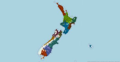
My data is in 12 feature classes, you can have any number. The pattern I will show works with data split into separate parts that can be processed concurrently. If your data is monolithic then either split it yourself spatially (oriented fishnet anyone?) or by adding a field signifying a batch identifier populated by row position - you can drop the field during processing.
I mentioned Snowflake, Big Query and Redshift warehouses. In all cases you can stage Parquet files where the target environment can see them and then load from the Parquet files. For spatial data, the Parquet files will need geometry encoded in a format understood by the target environment (Snowflake and Big Query support GeoJSON and WKT, Redshift supports WKT). I will only provide a worked example with GeoJSON going to Snowflake. My demo data is point geometry and the field I use to store the GeoJSON has a width of 100, if you are using polyline or polygon data you should investigate how wide your most point rich features are when encoding the field. For example I selected a very point rich polygon in a layer and as GeoJSON it is 2,071,156 characters:
with arcpy.da.SearchCursor('NZ Property Titles','shape@') as cursor:
    for row in cursor:
        print(len(str(row[0].__geo_interface__)))
2071156
Note that Data Interoperability can control the decimal precision used by GeoJSON; for geographic data a value of 7 is reasonable, the same polygon then uses 1,274,064 characters. For example the first coordinate goes from (172.90677540000001,-41.12752416699993) to (172.9067754,-41.1275242). Remember every byte counts!
Note: For Big Query, Data Interoperability has a GoogleBigQueryConnector hub transformer that can load CSV to tables. This may be simpler than sending Parquet and using the bq command environment to load data, I have not investigated the scenario.
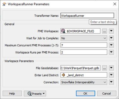
Let's dig into my particular workflow. The secret sauce is to create two ETL tools, the first marshals the jobs and calls a WorkspaceRunner transformer that calls the second tool, which does the work. It is very simple, here is LoadManager.fmw, it takes a list of arguments, in my case feature class names in a geodatabase:

WorkspaceRunner starts up to 7 FME processes that run a target tool until the job queue is consumed. Processing is likely to be CPU bound while worker processes extract, encode and upload the dataset files. I allowed each process to run two jobs which ate my incoming datasets in 6 processes.

Here is LoadWorkerParquet.fmw.

It also is a simple tool, it reads geodatabase, writes a local parquet file then sends the parquet file to Snowflake where the data is copied into a table. I'll let you inspect the SQLExecutor yourselves but as an aid to understanding, after variable substitution here is what a statement looks like (to Snowflake):
create or replace file format Canterburyparquet_format
  type = 'parquet';

create or replace temporary stage stageCanterbury
  file_format = Canterburyparquet_format;

put file://C:\Work\Parquet\TitlesCanterbury.parquet @stageCanterbury;

copy into "INTEROPERABILITY"."PUBLIC"."Titles"
  from (select
  $1:id::number,
  $1:title_no::varchar,
  $1:status::varchar,
  $1:type::varchar,
  $1:land_district::varchar,
  $1:issue_date::timestamp,
  $1:guarantee_status::varchar,
  $1:estate_description::varchar,
  $1:number_owners::varchar,
  $1:spatial_extents_shared::varchar,
  to_geography($1:geom::varchar)
  from @stageCanterbury);
Once the parquet file gets to Snowflake the ingest is blazing fast. By the way, I learned to do this by reading the help, I'm no Snowflake DBA.
What performance should you expect? At writing I'm trapped at home like the rest of us but on my home WiFi I get 2.3 million features loaded to Snowflake in 6 minutes, so with a decent computer and wired network I think conservatively 25 million point features per hour. Of course for a production environment and a really big job you could use multiple computers, certainly the target cloud warehouses will scale to take the throughput.
In the blog download you'll notice I include a second worker tool, LoadWorker.fmw, this was for me to compare performance of the usual way to write to Snowflake with 100K features per transaction, it was way slower.
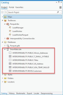
Now back in core Pro 2.9 my data is loaded to Snowflake and I can throw queries at it and enjoy the scaled compute experience.

I mentioned a Python option for creating parquet files, it is in the blog download but here it is too:
#  Pro 2.9+ example creation of a parquet file from a feature class
#  Geometry is encoded as GeoJSON in a field 'geom'

import arcpy
import pyarrow.parquet as pq
arcpy.env.overwriteOutput = True

#  Source feature class
Canterbury = r"C:\Work\Parquet\Parquet.gdb\Canterbury"

#  Create in-memory feature class in WGS84
with arcpy.EnvManager(outputCoordinateSystem='GEOGCS["GCS_WGS_1984",DATUM["D_WGS_1984",SPHEROID["WGS_1984",6378137.0,298.257223563]],PRIMEM["Greenwich",0.0],UNIT["Degree",0.0174532925199433]]',
                      geographicTransformations="NZGD_2000_To_WGS_1984_1"):
    arcpy.conversion.ExportFeatures(
        in_features=Canterbury,
        out_features=r"memory\Canterbury")

#  Add the geom field (non-point geometry will require a wider field
Canterbury = arcpy.management.AddField("memory\Canterbury","geom","TEXT",None,None,100,'',"NULLABLE","NON_REQUIRED",'').getOutput(0)

#  Derive GeoJSON
with arcpy.da.UpdateCursor(Canterbury,['shape@','geom']) as cursor:
    for row in cursor:
        row[1] = str(row[0].__geo_interface__)
        cursor.updateRow(row)

#  Drop geometry by creating a Table
esriTable = arcpy.conversion.TableToTable(Canterbury,"memory","CanterburyTable").getOutput(0)

#  Make arrow table
arrowTable = arcpy.da.TableToArrowTable(esriTable)

#  Write parquet
pq.write_table(arrowTable,r'C:\Work\Parquet\TitlesCanterbury.parquet',
               version='1.0',
               compression='SNAPPY')
Have fun moving that data around at scale!
You must be a registered user to add a comment. If you've already registered, sign in. Otherwise, register and sign in.