- Home
- :
- All Communities
- :
- Products
- :
- Data Management
- :
- Data Management Questions
- :
- Excel Question -Match Data from Two Excel Files th...
- Subscribe to RSS Feed
- Mark Topic as New
- Mark Topic as Read
- Float this Topic for Current User
- Bookmark
- Subscribe
- Mute
- Printer Friendly Page
Excel Question -Match Data from Two Excel Files that Share Similar Attributes
- Mark as New
- Bookmark
- Subscribe
- Mute
- Subscribe to RSS Feed
- Permalink
Hello,
I don't know if anyone knows this answer, but I thought I would give it a try here in our GeoNET. I need to do this first so that I can update it in GIS.
I have two different Excel spreadsheets. They have almost the same data, but it has been updated so some entries are not there anymore or some items have been added.
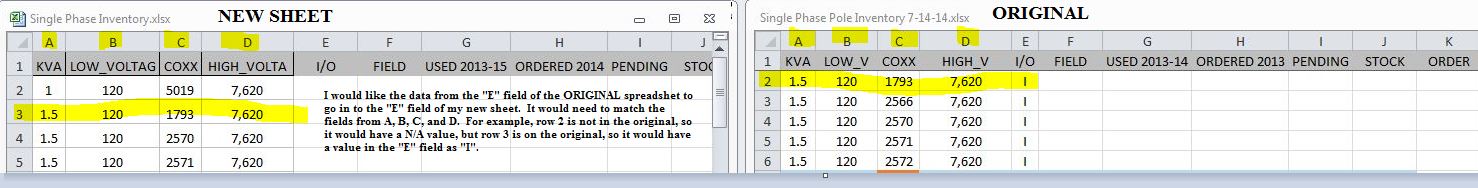
I have some items that are labeled "I" or "O" for inside or outside in the "E" columns. I need these in my new spreadsheet, and there are 300 or so of them.
The values that are the same and need to match are KVA, LOW_VOLTAGE,COXX, and HIGH_VOLTAGE (rows A, B, C, and D).
I would like to somehow have the formula look at these values from the original sheet, and if they are the same, it will put an "I" or "O" in the field "E" in my new sheet.
Thank you very much for helping me!
Solved! Go to Solution.
Accepted Solutions
- Mark as New
- Bookmark
- Subscribe
- Mute
- Subscribe to RSS Feed
- Permalink
In order to do this in Excel you would need to create a new column in both tables that concatenates the four look up columns together first. They you would use the VLookup formula to fill in column F (since you should insert the concatenated look up column into a new column A)
After inserting a new column A, the formula for the concatenation in cell A2 would be
=CONCATENATE(B2,";",C2,";",D2,";",E2)
Then drag this formula down the column to copy it and increase the row number
The VLookup formula would start in the new sheet's column F2 (I/O) and would be basically:
=VLOOKUP(A2,Sheet2!A$2:F$6,6,FALSE)
The F$6 portion of the formula should have the bold number edited to change it to the last filled in row number in the original sheet. Sheet2 should match the sheet name of the original data in your spreadsheet. Then drag this formula down the column to copy it and increase the A2 row number.
Convert the formulas to values before trying to open the spreadsheet in GIS, since GIS does not understand Excel formulas, only hard values.
- Mark as New
- Bookmark
- Subscribe
- Mute
- Subscribe to RSS Feed
- Permalink
Thank you for responding! I will try this out now and have it a go! I greatly greatly appreciate your response.
- Mark as New
- Bookmark
- Subscribe
- Mute
- Subscribe to RSS Feed
- Permalink
I don't think you need to add columns you can concatenate it all in a single formula, and output either I or O depending on whether there is an error.
Red text should point to your original sheet, replace the ... with the bottom row, and blue text should point to you new sheet. Ok?
=IF(ISERROR(CONCATENATE(VLOOKUP(A1,A$1:A$...,1,FALSE),(VLOOKUP(B1,B$1:B$...,1,FALSE)),(VLOOKUP(C1,C$1:C$...,1,FALSE)),(VLOOKUP(D1,D$1:D$...,1,FALSE)))),"O","I")
- Mark as New
- Bookmark
- Subscribe
- Mute
- Subscribe to RSS Feed
- Permalink
Ben:
Your suggestion will not work, since there are duplicate values in every individual column and only the first row with a given column value would be returned for each VLookup, which in most cases would have nothing to do with each other. Only the concatenation of all 4 columns will look up the correct row in the original spreadsheet. There is no way to do this without at least creating a new column in the original spreadsheet. Once that was done perhaps the VLookup could be written in the new sheet without adding a column, but that unnecessarily complicates the formula in a way that would waste my time with debugging unneeded complexity. The approach I suggested was easy to set up.
- Mark as New
- Bookmark
- Subscribe
- Mute
- Subscribe to RSS Feed
- Permalink
ugh,.... you're right, I had unique values in one of the columns in the test I set up.
I like to challenge myself with clean spreadsheets and dirty formulas.
- Mark as New
- Bookmark
- Subscribe
- Mute
- Subscribe to RSS Feed
- Permalink
Ben,
Thank you for responding to my questions. I'm grateful you even tried to help me!
- Mark as New
- Bookmark
- Subscribe
- Mute
- Subscribe to RSS Feed
- Permalink
Richard,
This worked perfectly! Thank you very much for your quick response. I just now had time to try it.