- Home
- :
- All Communities
- :
- ArcGIS Topics
- :
- Applications Prototype Lab
- :
- Applications Prototype Lab Blog
- :
- Raster Functions and the ArcGIS API for Python 1.2
Raster Functions and the ArcGIS API for Python 1.2
- Subscribe to RSS Feed
- Mark as New
- Mark as Read
- Bookmark
- Subscribe
- Printer Friendly Page
One of the great things about working in the Lab is you get to experiment with the new goodies from our core software developers before they are released. When I heard that version 1.2 of the ArcGIS API for Python would include a new module for raster functions, I could not wait to give it a try. Now that v.1.2 of the API is released, I can finally show you a Jupyter Notebook I built which has an example of a weighted overlay analysis implemented with raster functions. The following is a non-interactive version of that notebook which I exported to HTML. I hope it will give you some ideas for how you could use the ArcGIS API for Python to perform your own raster analysis.
Finding Natural and Accessible Areas in the State of Washington, USA
The weighted overlay is a standard GIS analysis technique for site-suitability and travel cost studies. This notebook leverages the new "arcgis.raster.functions" module in the ArcGIS API for Python 1.2 to demonstrate an example of a weighted overlay analysis. This example attempts to identify areas in the State of Washington that are "natural" while also being easy to travel within based on the following criteria:
- elevation (lower is better)
- steepness of the terrain (flatter is better)
- degree of human alteration of the landscape (less is better)
The input data for this analysis includes a DEM (Digital Elevation Model), and a dataset showing the degree of human modification to the landscape.
In general, weighted overlay analysis can be divided into three steps:
- Normalization: The pixels in the input raster datasets are reclassified to a common scale of numeric values based on their suitability according to the analysis criteria.
- Weighting: The normalized datasets are assigned a percent influence based on their importance to the final result by multiplying them by values ranging from 0.0 - 1.0. The sum of the values must equal 1.0.
- Summation: The sum of the weighted datasets is calculated to produce a final analysis result.
We'll begin by connecting to the GIS and accessing the data for the analysis.
Connect to the GIS
# import GIS from the arcgis.gis module
from arcgis.gis import GIS

# Connect to the GIS.
try:
   web_gis = GIS("https://dev004543.esri.com/arcgis", 'djohnsonRA')
   print("Successfully connected to {0}".format(web_gis.properties.name))
except:
   print("")
Enter password:········
Successfully connected to ArcGIS Enterprise A
Search the GIS for the input data for the analysis
Human Modified Index
# Search for the Human Modified Index imagery layer item by title
item_hmi = web_gis.content.search('title:Human Modified Index', 'Imagery Layer')[0]
item_hmi
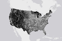
A measure of the degree of human modification, the index ranges from 0.0 for a virgin landscape condition to 1.0, for the most heavily modified areas.
Last Modified: July 06, 2017
0 comments, 2 views
Elevation
# Search for the DEM imagery layer item by title
item_dem = web_gis.content.search('title:USGS NED 30m', 'Imagery Layer')[0]
item_dem
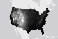
The National Elevation Dataset (NED) is the primary elevation data product of the USGS. This version was resampled to 30m from source data at 1/3 arc-second resolution and projected to an Albers Equal Area coordinate system.
Last Modified: July 06, 2017
0 comments, 8 views
Study area boundary and extent
# Search for the Ventura County feature layer item by title
item_studyarea = web_gis.content.search('title:State of Washington, USA',
                                        'Feature Layer')[0]
item_studyarea
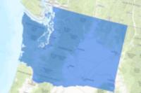
State of Washington, USA
Last Modified: July 07, 2017
0 comments, 2 views
# Get a reference to the feature layer from the portal item
lyr_studyarea = item_studyarea.layers[0]
lyr_studyarea
<FeatureLayer url:"https://dev004543.esri.com/server/rest/services/Hosted/Washington/FeatureServer/1">
Get the coordinate geometry of the study area
# Query the study area layer to get the boundary feature
query_studyarea = lyr_studyarea.query(where='1=1')
# Get the coordinate geometry of the study area.
# The geometry will be used to extract the Elevation and Human Modified Index data.
geom_studyarea = query_studyarea.features[0].geometry
# Set the spatial reference of the geometry.
geom_studyarea['spatialReference'] = query_studyarea.spatial_reference
Get the extent of the study area
# Import the geocode function
from arcgis.geocoding import geocode
# Use the geocode function to get the location/address of the study area
geocode_studyarea = geocode('State of Washington, USA',
                            out_sr= query_studyarea.spatial_reference)
# Get the geographic extent of the study area
# This extent will be used when displaying the Elevation, Human Modified Index,
# and final result data.
extent_studyarea = geocode_studyarea[0]['extent']
extent_studyarea
{'xmax': -1451059.3770040546,
'xmin': -2009182.5321227335,
'ymax': 1482366.818700374,
'ymin': 736262.260048952}
Display the analysis data
Human Modified Index
# Get a reference to the imagery layer from the portal item
lyr_hmi = item_hmi.layers[0]
# Set the layer extent to geographic extent of study area and display the data.
lyr_hmi.extent = extent_studyarealyr_hmi

Elevation
# Get a reference to the imagery layer from the portal item
lyr_dem = item_dem.layers[0]
# Set the layer extent to the geographic extent of study area and display the data.
lyr_dem.extent = extent_studyarealyr_dem

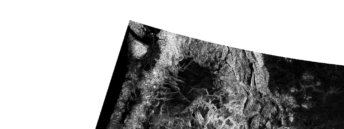
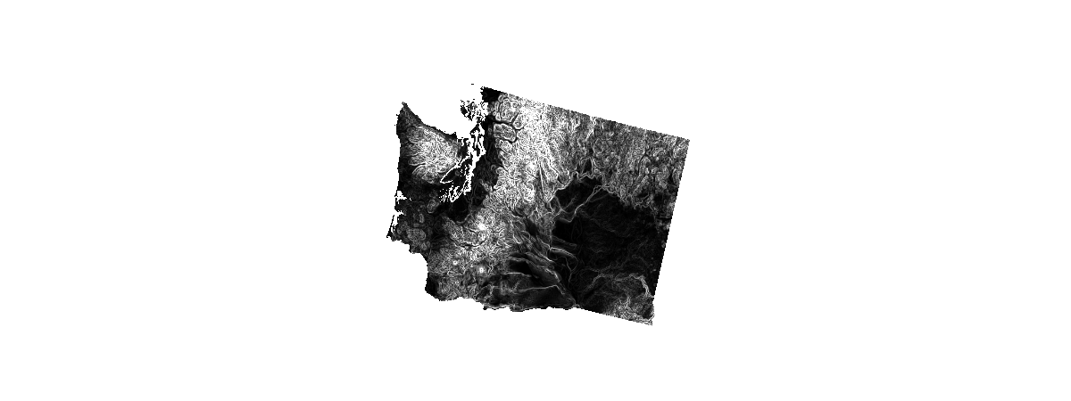
Slope (derived from elevation via the Slope raster function)
# Import the raster functions from the ArcGIS API for Python (new to version 1.2!)
from arcgis.raster.functions import *
# Derive a slope layer from the DEM layer using the slope function
lyr_slope = slope(dem=lyr_dem,slope_type='DEGREE', z_factor=1)
# Use the stretch function to enhance the display of the slope layer.
lyr_slope_stretch = stretch(raster=lyr_slope, stretch_type='StdDev', dra='true')
# Display the stretched slope layer within the extent of the study area.
lyr_slope_stretch.extent= extent_studyarealyr_slope_stretch
Extract the data within the study area geometry
Use the Clip raster function to extract the analysis data from within the study area geometry
Human Modified Index
# Extract the Human Modified Index data from within the study area geometry
hmi_clipped = clip(raster=lyr_hmi, geometry=geom_studyarea)
hmi_clipped

Elevation#Elevation
# Extract the Elevation data from within the study area geometry
elev_clipped = clip(raster=lyr_dem, geometry=geom_studyarea)
elev_clipped

Slope#Slope
# Extract the Slope data from within the study area geometry
slope_clipped = clip(raster=lyr_slope, geometry=geom_studyarea)
# Apply the Stretch function to enhance the display of the slope_clipped layer.
slope_clipped_stretch = stretch(raster=slope_clipped, stretch_type='StdDev',
                                dra='true')
slope_clipped_stretch
Perform the analysis
Step 1: Normalization
Use the Remap function to normalize each set of input data to a common scale of 1 - 9, where 1 = least suitable and 9 = most suitable.

# Create a colormap to display the analysis results with 9 colors ranging
# from red to yellow to green.
clrmap=  [[1, 230, 0, 0], [2, 242, 85, 0], [3, 250, 142, 0], [4, 255, 195, 0],
         [5, 255, 255, 0], [6, 197, 219, 0], [7, 139, 181, 0], [8, 86, 148, 0],
         [9, 38, 115, 0]]
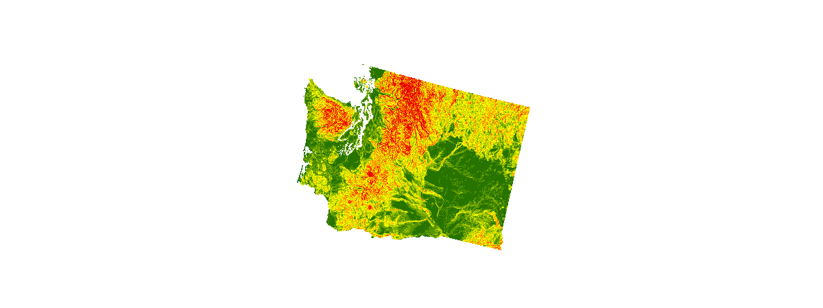
# Normalize the elevation data
elev_normalized = remap(raster=elev_clipped,
                        input_ranges=[0,490, 490,980, 980,1470, 1470,1960, 1960,2450,
                                      2450,2940, 2940,3430, 3430,3700, 3920,4100],
                        output_values=[9,8,7,6,5,4,3,2,1], astype='U8')

# Display color-mapped image of the reclassified elevation data
colormap(elev_normalized, colormap=clrmap)

# Normalize the slope data
slope_normalized = remap(raster=slope_clipped,
                        input_ranges=[0,1, 1,2, 2,3, 3,5, 5,7, 7,9, 9,12, 12,15,
                                      15,100],
                        output_values=[9,8,7,6,5,4,3,2,1],  astype='U8')

# Display a color-mapped image of the reclassified slope data
colormap(slope_normalized, colormap=clrmap)
# Normalize the Human Modified Index data
hmi_normalized = remap(raster=hmi_clipped,
                      input_ranges=[0.0,0.1, 0.1,0.2, 0.2,0.3, 0.3,0.4, 0.4,0.5,
                                    0.5,0.6, 0.6,0.7, 0.7,0.8, 0.8,1.1],
                      output_values=[9,8,7,6,5,4,3,2,1],  astype='U8')

# Display a color-mapped image of the reclassified HMI data
colormap(hmi_normalized, colormap=clrmap)

Step 2: Weighting
Use the overloaded multiplication operator * to assign a weight to each normalized dataset based on their relative importance to the final result.
# Apply weights to the normalized data using the overloaded multiplication
# operator "*".
# - Human Modified Index: 60%
# - Slope: 25%
# - Elevation: 15%
hmi_weighted = hmi_normalized * 0.6
slope_weighted = slope_normalized * 0.25
elev_weighted = elev_normalized * 0.15
Step 3: Summation
Add the weighted datasets together to produce a final analysis result.
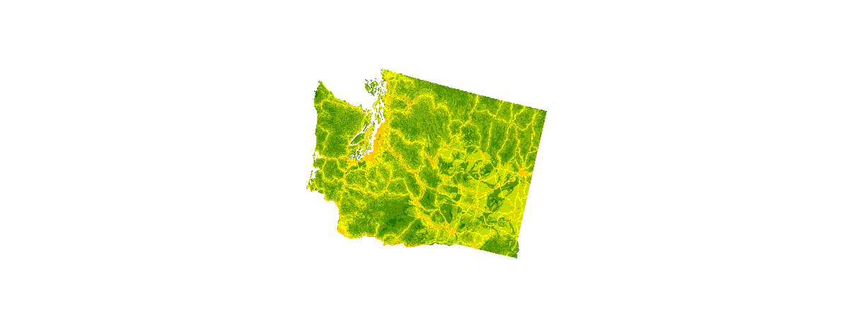
# Calculate the sum of the weighted datasets using the overloaded addition
# operator "+".
result_dynamic = colormap(hmi_weighted + slope_weighted + elev_weighted,
                          colormap=clrmap, astype='U8')
result_dynamic
The same analysis can also be performed in a single operation
result_dynamic_one_op = colormap(
   raster=
   (
      # Human modified index layer
      0.60 * remap(raster=clip(raster=lyr_hmi, geometry=geom_studyarea),
         input_ranges=[0.0,0.1, 0.1,0.2, 0.2,0.3, 0.3,0.4, 0.4,0.5,
                       0.5,0.6, 0.6,0.7, 0.7,0.8, 0.8,1.1],
         output_values=[9,8,7,6,5,4,3,2,1])
      +
      # Slope layer
      0.25 * remap(raster=clip(raster=lyr_slope, geometry=geom_studyarea),
         input_ranges=[0,1, 1,2, 2,3, 3,5, 5,7, 7,9, 9,12, 12,15,
                       15,100],
         output_values=[9,8,7,6,5,4,3,2,1])
      +
      # Elevation layer
      0.15 * remap(raster=clip(raster=lyr_dem, geometry=geom_studyarea),
         input_ranges=[-90,250, 250,500, 500,750, 750,1000, 1000,1500,
                       1500,2000, 2000,2500, 2500,3000, 3000,5000],
         output_values=[9,8,7,6,5,4,3,2,1])
   ),
   colormap=clrmap,  astype='U8')
result_dynamic_one_op
Generate a persistent analysis result via distributed server based raster processing.
Portal for ArcGIS has been enhanced with the ability to perform distributed server based processing on imagery and raster data. This technology enables you to boost the performance of raster processing by processing data in a distributed fashion, even at full resolution and full extent.
You can use the processing capabilities of ArcGIS Pro to define the processing to be applied to raster data and perform processing in a distributed fashion using their on premise portal. The results of this processing can be accessed in the form of a web imagery layer that is hosted in their ArcGIS Organization.
For more information, see Raster analysis on Portal for ArcGIS
# Does the GIS support raster analytics?
import arcgis
arcgis.raster.analytics.is_supported(web_gis)
True
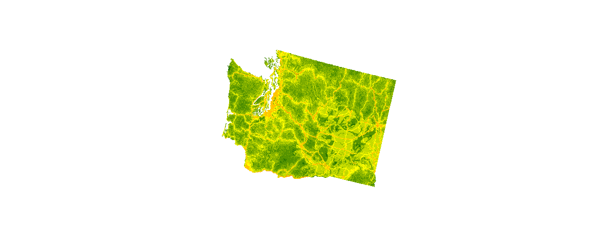
# The .save() function invokes generate_raster from the arcgis.raster.analytics
# module to run the analysis on a GIS server at the source resolution of the
# input datasets and store the result as a persistent web imagery layer in the GIS.
result_persistent = result_dynamic.save("NaturalAndAccessible_WashingtonState")
result_persistent

Analysis Image Service generated from GenerateRaster
Last Modified: July 07, 2017
0 comments, 0 views
# Display the persistent result
lyr_result_persistent = result_persistent.layers[0]
lyr_result_persistent.extent = extent_studyarea
lyr_result_persistent

You must be a registered user to add a comment. If you've already registered, sign in. Otherwise, register and sign in.