- Home
- :
- All Communities
- :
- Developers
- :
- Python
- :
- Python Questions
- :
- Trend Analysis Through Time Series of Raster Data
- Subscribe to RSS Feed
- Mark Topic as New
- Mark Topic as Read
- Float this Topic for Current User
- Bookmark
- Subscribe
- Mute
- Printer Friendly Page
Trend Analysis Through Time Series of Raster Data
- Mark as New
- Bookmark
- Subscribe
- Mute
- Subscribe to RSS Feed
- Permalink
Hi All,
I have total 13 raster files for different years (2001 - 2013). All data are in tiff format and same spatial extent (row and column). I am trying to perform regression line slope/trend analysis between each grid points for 13 raster data sets. I have tried in ArcGIS raster calculator but I won't run the task due to complexity.
The outcome would measure the net change between pixels through my time series data.
So my question is, can it be performed using raster calculator or ArcPy Script? For such type of statistical analysis using ArcGIS, really I am facing one of the big limitation with ArcGIS.
Using excel, it can be calculated using SLOPE command where X (Time) and Y (value) has been used. But for creating a Spatial map of Slope/trend analysis, we need to perform using raster data.
The download link is given below for Sample data sets (Due to size limit, I could not attach the data with here )
Data Link: Dropbox - Water_Use_Efficiency.zip
Please share your experience.
Thanks in advance.
Solved! Go to Solution.
Accepted Solutions
- Mark as New
- Bookmark
- Subscribe
- Mute
- Subscribe to RSS Feed
- Permalink
I also came across this tool: Curve Fit : A Pixel Level Raster Regression Tool - Desktop Decision Support Tools by the USGS
- Mark as New
- Bookmark
- Subscribe
- Mute
- Subscribe to RSS Feed
- Permalink
Xander Bakker Patterson , A request to you peoples, We need your kind cooperation to solve the issue. Since long i am trying but not solved yet. Thanks
- Mark as New
- Bookmark
- Subscribe
- Mute
- Subscribe to RSS Feed
- Permalink
Hishouvik jha ,
Recently I needed to detect strange behavior in monthly consumption by water consumers. I created a data structure that had the 12 months of data for each client as attributes of a point file. The code below is a snippet that takes a list of data (this could be the 13 values for each pixel in your case) and calculates a regression line based on the data.
The slope will tell you if there is an increase or decrease in the range of data. In my case to detect this abnormal behavior I determined the average value, and the mean distance for each value to the regression line divided by mean value. The higher the value the less constant the consumption.
I think you could use this code (or parts) to create the numpy arrays for each raster and loop through the individual pixels (create a list of values for the 13 years you have for each pixel, do the calculation and fill an output array to write the result of the analysis to an output raster. I'm pretty sure there must be an easier way to do this, or even a standard way to calculate this on a time series of data. I will investigate a little more and let you know.
from numpy import arange,array,ones,linalg
def main():
# some test input data (lists of 12 elements with possible NoData)
lst_data = [[2.0, None, None, None, None, 1.0, 4.0, 6.0, 5.0, 7.0, 9.0, 9.0],
[None, None, None, None, None, None, None, None, None, None, 15.0, 16.0],
[14.0, 11.0, 25.0, 4.0, 4.0, 4.0, 3.0, 4.0, 2.0, 3.0, 4.0, 4.0],
[7.0, 9.0, 7.0, 3.0, 2.0, 2.0, None, 13.0, 5.0, 60.0, 25.0, 25.0],
[1.0, 2.0, 3.0, 4.0, 5.0, 6.0, 7.0, 8.0, 9.0, 10.0, 11.0, 12.0],
[1.0, 2.0, 1.0, 2.0, 1.0, 2.0, 1.0, 2.0, 1.0, 2.0, 1.0, 2.0],
[11.0, 12.0, 11.0, 12.0, 11.0, 12.0, 11.0, 12.0, 11.0, 12.0, 11.0, 12.0]]
# loop through input data
for lst in lst_data:
print "\ndata:", lst
# calculate regression line: y = ax + b
a, b, sum_abs_dif, avg_abs_dif = RegressionLine(lst)
if not a is None:
cons_prom = getAvg(lst)
print " - mean value:", cons_prom
print " - slope (a):", a
print " - intercept (b):", b
print " - total distance from regression line:", sum_abs_dif
print " - mean distance from regression line :", avg_abs_dif
# print a, b, sum_abs_dif, avg_abs_dif
print " - score:", avg_abs_dif / cons_prom
else:
print " - Insufficient data"
def RegressionLine(lst):
from numpy import arange, array, ones, linalg
months = range(1, 13)
lst_x = []
lst_y = []
cnt = 0
for a in lst:
if not a is None:
lst_x.append(months[cnt])
lst_y.append(a)
cnt += 1
cnt_elem = len(lst_x)
if cnt_elem >= 2:
A = array([ lst_x, ones(len(lst_x))])
# linearly generated sequence
w = linalg.lstsq(A.T, lst_y)[0]
# obtaining the parameters of the regression line
a = w[0] # slope
b = w[1] # offset
# calculate acumulated abs difference from trend line
zip_lst = zip(lst_x, lst_y)
sum_abs_dif = 0
for xy in zip_lst:
x = xy[0]
y = xy[1]
calc = x * a + b
abs_dif = abs(y - calc)
sum_abs_dif += abs_dif
avg_abs_dif = sum_abs_dif / cnt_elem
return a, b, sum_abs_dif, avg_abs_dif
else:
return None, None, None, None
def getAvg(lst):
corr_lst = [a for a in lst if not a is None]
cnt = len(corr_lst)
if cnt == 0:
return None
else:
return sum(corr_lst) / float(cnt)
if __name__ == '__main__':
main()Results:
data: [2.0, None, None, None, None, 1.0, 4.0, 6.0, 5.0, 7.0, 9.0, 9.0]
- mean value: 5.375
- slope (a): 0.738095238095
- intercept (b): -0.529761904762
- total distance from regression line: 9.29761904762
- mean distance from regression line : 1.16220238095
- score: 0.216223698782
data: [None, None, None, None, None, None, None, None, None, None, 15.0, 16.0]
- mean value: 15.5
- slope (a): 1.0
- intercept (b): 4.0
- total distance from regression line: 3.5527136788e-15
- mean distance from regression line : 1.7763568394e-15
- score: 1.14603667058e-16
data: [14.0, 11.0, 25.0, 4.0, 4.0, 4.0, 3.0, 4.0, 2.0, 3.0, 4.0, 4.0]
- mean value: 6.83333333333
- slope (a): -1.18181818182
- intercept (b): 14.5151515152
- total distance from regression line: 42.303030303
- mean distance from regression line : 3.52525252525
- score: 0.515890613452
data: [7.0, 9.0, 7.0, 3.0, 2.0, 2.0, None, 13.0, 5.0, 60.0, 25.0, 25.0]
- mean value: 14.3636363636
- slope (a): 2.69171974522
- intercept (b): -3.0101910828
- total distance from regression line: 103.946496815
- mean distance from regression line : 9.44968152866
- score: 0.65788922035
data: [1.0, 2.0, 3.0, 4.0, 5.0, 6.0, 7.0, 8.0, 9.0, 10.0, 11.0, 12.0]
- mean value: 6.5
- slope (a): 1.0
- intercept (b): -1.46316339947e-15
- total distance from regression line: 3.17523785043e-14
- mean distance from regression line : 2.64603154202e-15
- score: 4.07081775696e-16
data: [1.0, 2.0, 1.0, 2.0, 1.0, 2.0, 1.0, 2.0, 1.0, 2.0, 1.0, 2.0]
- mean value: 1.5
- slope (a): 0.020979020979
- intercept (b): 1.36363636364
- total distance from regression line: 5.87412587413
- mean distance from regression line : 0.48951048951
- score: 0.32634032634
data: [11.0, 12.0, 11.0, 12.0, 11.0, 12.0, 11.0, 12.0, 11.0, 12.0, 11.0, 12.0]
- mean value: 11.5
- slope (a): 0.020979020979
- intercept (b): 11.3636363636
- total distance from regression line: 5.87412587413
- mean distance from regression line : 0.48951048951
- score: 0.042566129522- Mark as New
- Bookmark
- Subscribe
- Mute
- Subscribe to RSS Feed
- Permalink
I also came across this tool: Curve Fit : A Pixel Level Raster Regression Tool - Desktop Decision Support Tools by the USGS
- Mark as New
- Bookmark
- Subscribe
- Mute
- Subscribe to RSS Feed
- Permalink
Hi Xander Bakker, Thank you.
The script is quite interesting. in above script, there are seven client's data has been used for the analysis. Instead of using a numeric value which you assigned as an input data, it can be possible to assign raster file or ASC file in there? If is it possible to use raster or ASC file as an input data then output also can be written in raster format. (Plz give your opinion also)
Somewhere I have read that if we stack all the year's data and make it a single raster. Might be it will help us to perform a loop on all pixels (number of the pixels at same grid point for all years, so in my case at the same grid point, the number of pixels is 13) at same grid point for the raster based statistical analysis such as trend, correlation etc.
basically, Since long the geospatial research communities are also looking for the same analysis on Python or ArcGIS raster calculator platform, as following
1) Raster based Trend Analysis through time series data.
2) Raster based correlation analysis between two variables. Just assume the correlation analysis between Temperature and precipitation raster data and output also be in raster format.
If the above issues can be solved on Python platform so it would be a very good news for all researchers who are looking for the solution since long.
The tool which you suggested, It is very helpful and the number of functions is inbuilt with the tool but the only issue is, it is only functioning on ArcGIS 10.1 version. It is not compatible with the later version of ArcGIS 10.1 and taking too long time for the analysis. However, I am going through with that tool. In addition, I am trying to further explore the script which you provided.
It is our kind request behalf of the geospatial research community, India, please show a path to overcome the issues. If you need the sample data, I can provide you some datasets for further investigation on the matter.
Once again thank you very much for your cooperation.
With warm regards
Shouvik Jha
- Mark as New
- Bookmark
- Subscribe
- Mute
- Subscribe to RSS Feed
- Permalink
Hi shouvik jha ,
For your first question, is it possible to connect to a datasource, the answer is yes. In my case the data was available as point data and the 12 values as 12 fields for each feature. I read them into a list of values and process the results and write the output statistic values to additional field in the point feature class.
In your case you have a list of 13 raster where each raster aligns with the other raster and the number of rows and columns match. You will have to loop through each pixel location in a numpy array that was created from converting the each raster to a numpy, and for each pixel location you will read the 13 values out (from the 13 numpy arrays), construct the list, perform the analysis and populate a new numpy array as the output result.
It would be interesting to have access to the 13 rasters to see what can be done. So if you can share them, please attach them at the thread.
You could also explore the How Band Collection Statistics works—Help | ArcGIS Desktop tool, although this will not create a raster as a result, but a report using the pixels in a diagonal of the bands (you will need to check the "compute covariance and correlation matrices" option).
- Mark as New
- Bookmark
- Subscribe
- Mute
- Subscribe to RSS Feed
- Permalink
Hi Xander Bakker, Thank you.
I have attached the Dropbox link at the thread for accessing the data. Due to the size limit, I could not attach the data with here, however, you can download the data by that link and please have a look.
- Mark as New
- Bookmark
- Subscribe
- Mute
- Subscribe to RSS Feed
- Permalink
You shouldn't have to cycle through the cells of a stacked raster .... consider
# ---- create a 'raster' consisting of 4 rows and 5 columns with 12
# months of data... ie. 12 months x 4 rows x 5 columns
a = np.arange(12*4*5).reshape(12, 4, 5)
a[0] # ---- the first month
array([[ 0, 1, 2, 3, 4],
[ 5, 6, 7, 8, 9],
[10, 11, 12, 13, 14],
[15, 16, 17, 18, 19]])
a[-1] # ---- the last month ..... you get the drift I hope
array([[220, 221, 222, 223, 224],
[225, 226, 227, 228, 229],
[230, 231, 232, 233, 234],
[235, 236, 237, 238, 239]])
top_left_12months = a[:, 0, 0] # --- let's get the top-left cell's data
array([ 0, 20, 40, ..., 180, 200, 220]) # ---- makes sense doesn't it?
np.mean(top_left_12months) # ---- the 12 month mean for the top left cell
110.0
np.mean(a, axis=0) # ---- Since I am lazy, I will get every cell's average
array([[ 110.00, 111.00, 112.00, 113.00, 114.00],
[ 115.00, 116.00, 117.00, 118.00, 119.00],
[ 120.00, 121.00, 122.00, 123.00, 124.00],
[ 125.00, 126.00, 127.00, 128.00, 129.00]])
# ---- Notice the top left cell value is correct
#The point being,... once you snag the data you can do anything you want to it. In the above example, I simply used a builtin function to calculate the mean... that doesn't mean that I am restricted to using builtin functions. The possibilities are endless since calculations can be 'vectorized' in any dimension... in this case, by row, by column or by depth/band/month/whatever is the 3rd dimension.
PS handling nodata values is trivial when working with arrays... in fact, many are builtin... instead of np.mean... there is amazingly ... np.nanmean()
- Mark as New
- Bookmark
- Subscribe
- Mute
- Subscribe to RSS Feed
- Permalink
Thanks, Dan_Patterson, I am trying to further explore the script.
- Mark as New
- Bookmark
- Subscribe
- Mute
- Subscribe to RSS Feed
- Permalink
See below an example which I created from the slope of the regression line based on the 13 values. This means that if the values increment in time they will have a positive slope (red) and in case of a decreasing regression line a negative slope (green):
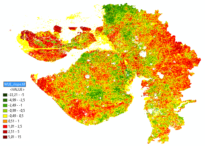
The code used to create this raster is:
#-------------------------------------------------------------------------------
# Name: stats_numpy_series.py
# Purpose:
#
# Author: Xander
#
# Created: 30-07-2017
#-------------------------------------------------------------------------------
def main():
print "load modules..."
import arcpy
import numpy as np
# template = r'C:\GeoNet\LoopMultiFolderCalcMeanSameFolder\Test_Data\2004A\{0}162004.tif'
template = r'C:\GeoNet\WUE\r{0}_WUE.TIF'
nodata = -3.4028235e+38
out_ras = r'C:\GeoNet\WUE\WUE_slope.tif'
print "create numpy list..."
lst_np_ras = []
for i in range(1, 14):
ras_path = template.format("%03d" % (i,))
print " - ", ras_path
ras_np = arcpy.RasterToNumPyArray(ras_path)
lst_np_ras.append(ras_np)
print "read props numpy raster..."
ras_np = lst_np_ras[0]
rows = ras_np.shape[0]
cols = ras_np.shape[1]
print "create output numpy array..."
ras_path = template.format("%03d" % (1,))
raster = arcpy.Raster(ras_path)
ras_np_res = np.ndarray((rows, cols)) # np.ndarray((raster.height, raster.width))
print "loop through pixels..."
pix_cnt = 0
for row in range(rows):
for col in range(cols):
pix_cnt += 1
if pix_cnt % 10000 == 0:
print "row:", row, " col:", col, " pixel:", pix_cnt
lst_vals = []
for ras_np in lst_np_ras:
lst_vals.append(ras_np[row, col])
lst_vals = ReplaceNoData(lst_vals, nodata)
# perform calculation on list
a, b, sum_abs_dif, avg_abs_dif, cnt_elem = RegressionLine(lst_vals)
if cnt_elem > 1:
val = a
## print " - ", lst_vals
## print " - slope (a):", a
## print " - intercept (b):", b
## print " - total distance from regression line:", sum_abs_dif
## print " - mean distance from regression line :", avg_abs_dif
else:
val = nodata
try:
ras_np_res[row, col] = val
except:
print "err"
pnt = arcpy.Point(raster.extent.XMin, raster.extent.YMin)
xcellsize = raster.meanCellWidth
ycellsize = raster.meanCellHeight
ras_res = arcpy.NumPyArrayToRaster(ras_np_res, lower_left_corner=pnt, x_cell_size=xcellsize,
y_cell_size=ycellsize, value_to_nodata=nodata)
ras_res.save(out_ras)
arcpy.DefineProjection_management(in_dataset=out_ras, coor_system="GEOGCS['GCS_WGS_1984',DATUM['D_WGS_1984',SPHEROID['WGS_1984',6378137.0,298.257223563]],PRIMEM['Greenwich',0.0],UNIT['Degree',0.0174532925199433]]")
def ReplaceNoData(lst, nodata):
res = []
for a in lst:
if a < nodata / 2.0:
res.append(None)
else:
res.append(a)
return res
def RegressionLine(lst):
from numpy import arange, array, ones, linalg
months = range(1, 14)
lst_x = []
lst_y = []
cnt = 0
for a in lst:
if not a is None:
lst_x.append(months[cnt])
lst_y.append(a)
cnt += 1
cnt_elem = len(lst_x)
if cnt_elem >= 2:
A = array([ lst_x, ones(len(lst_x))])
# linearly generated sequence
w = linalg.lstsq(A.T, lst_y)[0]
# obtaining the parameters of the regression line
a = w[0] # slope
b = w[1] # offset
# calculate acumulated abs difference from trend line
zip_lst = zip(lst_x, lst_y)
sum_abs_dif = 0
for xy in zip_lst:
x = xy[0]
y = xy[1]
calc = x * a + b
abs_dif = abs(y - calc)
sum_abs_dif += abs_dif
avg_abs_dif = sum_abs_dif / cnt_elem
return a, b, sum_abs_dif, avg_abs_dif, cnt_elem
else:
return None, None, None, None, None
if __name__ == '__main__':
main()
I have attached the raster for you to examine.
Kind regards, Xander