- Home
- :
- All Communities
- :
- Developers
- :
- Python
- :
- Python Questions
- :
- numpy linalg.lstsq - coordinate translations
- Subscribe to RSS Feed
- Mark Topic as New
- Mark Topic as Read
- Float this Topic for Current User
- Bookmark
- Subscribe
- Mute
- Printer Friendly Page
numpy linalg.lstsq - coordinate translations
- Mark as New
- Bookmark
- Subscribe
- Mute
- Subscribe to RSS Feed
- Permalink
I have some control points from a local grid to a known grid (a national grid system).
What I am trying to do is come up with the appropriate parameters to define a local prj for the input data.
This involves finding the origin (or rotation point), the amount of rotation, and any shifts or scaling in X & Y.
So, I have been messing with this code found here :
how-to-perform-coordinates-affine-transformation-using-python-part-2
So, what I have got is (almost the same as the referenced post 😞
import sys, os
import numpy as np
localData = [["AJP1", 5671.666, 19466.156], ["GCP CR", 9634.659, 13064.567], \
["MHP2", 10325.093, 7797.802], ["MILE 8", 6508.217, 7511.953]]
refData =[["AJP1", 157171.409, 75402.914], ["GCP CR", 158414.820, 67978.050], \
["MHP2", 157059.513, 62842.546], ["MILE 8", 153418.976, 64023.272]]
inArr = np.array([[l[1], l[2], 0.0] for l in localData])
refArr = np.array([[l[1], l[2], 0.0] for l in refData])
n = inArr.shape[0]
pad = lambda x: np.hstack([x, np.ones((x.shape[0], 1))])
unpad = lambda x: x[:,:-1]
X = pad(inArr)
Y = pad(refArr)
# Solve the least squares problem X * A = Y
# to find our transformation matrix A
A, res, rank, s = np.linalg.lstsq(X, Y)
transform = lambda x: unpad(np.dot(pad(x), A))
print "Target:"
print refArr
print "Result:"
print transform(inArr)
print "Max error:", np.abs(refArr - transform(inArr)).max()which give me this :
>>>
Target:
[[ 157171.409 75402.914 0. ]
[ 158414.82 67978.05 0. ]
[ 157059.513 62842.546 0. ]
[ 153418.976 64023.272 0. ]]
Result:
[[ 157171.39578228 75402.91459879 0. ]
[ 158414.84986487 67978.04864706 0. ]
[ 157059.48564043 62842.54723945 0. ]
[ 153418.98671243 64023.2715147 0. ]]
Max error: 0.0298648653843So, I can see the fit is quite good.
But how do I use the solution from np.linalg.lstsq to derive the parameters I need for the projection definition of the localData?
In particular, the origin point 0,0 in the target coordinates, and the shifts and rotations that are going on here??
Tagging out very own numpy expert and all around math wiz Dan Patterson here.
Or is this not even possible with this approach.
My matrix math is extremely rusty to non-existent. But I am willing to try any methods offered 
Thanks in advance.
Neil
- Mark as New
- Bookmark
- Subscribe
- Mute
- Subscribe to RSS Feed
- Permalink
Yes... I think I have one nostril above water...how about providing a coordinate list of 'from' and 'to' points so I can check with real world coordinates. If you want, post here and/or email me at my uni email on my profile page.
- Mark as New
- Bookmark
- Subscribe
- Mute
- Subscribe to RSS Feed
- Permalink
Dan, thanks for your help on this...
Well a representative sample are those 4 points I posted originally. The local points are from a rotated project grid.
And the refPoints are as measured using the national grid system (which is normally oriented). Both are on the same classical datum for the area. The datum transformation dosn't come into this.
I have other examples here, but these are good enough I think.
The code I found give me a good idea of the overall fit of the points, and will enable me to identify any points which are way off because of measurement or transcription errors. I was just trying to come up with a method that would enable me to describe a local coordinate system - origin point, rotation and scale, to correctly define this system in an ArcGIS prj.
- Mark as New
- Bookmark
- Subscribe
- Mute
- Subscribe to RSS Feed
- Permalink
And, in the original code I found, why do i need the extra 0.0 in the array before that pad lambda function?
Never use those, cos i can't get my brain around them....
- Mark as New
- Bookmark
- Subscribe
- Mute
- Subscribe to RSS Feed
- Permalink
An affine transformation is a combination of a translation, scaling and rotation transformations, which can be expressed as:
[1 0 tx] [Sx 0 0] [cos(a) -sin(a) 0] [a b c]
A = [0 1 ty] . [0 Sy 0] . [sin(a) cos(a) 0] = [d e f]
[0 0 1 ] [0 0 1] [0 0 1] [0 0 1]
the extra 0 is for use with homogenous coordinates. There are several ways of accomplishing the same thing
>>> a
array([[ 1.00000000, 1.00000000],
[ 2.00000000, 2.00000000],
[ 3.00000000, 3.00000000],
[ 4.00000000, 4.00000000],
[ 5.00000000, 5.00000000]])
>>> b = affine(a, angle=-45)[0]
>>> c = affine(a, 45)[0]
>>> b
array([[ 0.17157288, 3.00000000],
[ 1.58578644, 3.00000000],
[ 3.00000000, 3.00000000],
[ 4.41421356, 3.00000000],
[ 5.82842712, 3.00000000]])
>>> c
array([[ 3.00000000, 0.17157288],
[ 3.00000000, 1.58578644],
[ 3.00000000, 3.00000000],
[ 3.00000000, 4.41421356],
[ 3.00000000, 5.82842712]])Where the simplied version drops the last row and right-most column as was done in the above example
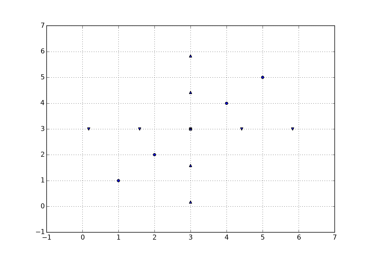
'a' is the points at a 45 degree angle at a 45 degree (circles). 'b' is rotated -45 (parallel to x) and 'c' parallel to y.
All are centered about the point (3,3) which is the center of input points. All points are translated (moved to the
origin, then rotated, then translated back to their original center.
# array 'a' is pnts in the examples below
# rotation is the angle in degrees
#
#translate....
p_trans = pnts - cent_pnt(pnts)
a_c = np.average(a, axis=0).squeeze() # cent_pnt is basically this
#
#rotation matrix....
rad = np.deg2rad(rotation)
c = np.cos(rad)
s = np.sin(rad)
rot_mat = np.array([[c, -s], [s, c]])
#
#rotate the translated points, get the dot product, take its translation and move back
p_rot = np.dot(rot_mat, p_trans.T).T + to_pntA rigid 2d Affine essentially.
>>> a # input array
array([[ 1.00000000, 1.00000000],
[ 2.00000000, 2.00000000],
[ 3.00000000, 3.00000000],
[ 4.00000000, 4.00000000],
[ 5.00000000, 5.00000000]])
>>> a.T # translated .... from column to row for x, y values
array([[ 1.00000000, 2.00000000, 3.00000000, 4.00000000, 5.00000000],
[ 1.00000000, 2.00000000, 3.00000000, 4.00000000, 5.00000000]])
>>> a_c # the center of 'a'
array([ 3.00000000, 3.00000000])
>>> a_h # the coordinates translated to the center
array([[-2.00000000, -2.00000000],
[-1.00000000, -1.00000000],
[ 0.00000000, 0.00000000],
[ 1.00000000, 1.00000000],
[ 2.00000000, 2.00000000]])
>>> a_h.T # translate those to rows so that you can use the dot product
array([[-2.00000000, -1.00000000, 0.00000000, 1.00000000, 2.00000000],
[-2.00000000, -1.00000000, 0.00000000, 1.00000000, 2.00000000]])
>>>
>>> rm # a rotation matrix for a 45 degree rotation
array([[ 0.70710678, 0.70710678],
[-0.70710678, 0.70710678]])
>>>
>>> np.dot(rm, a_h.T).T # from the calc. class we all skipped
array([[-2.82842712, -0.00000000],
[-1.41421356, -0.00000000],
[ 0.00000000, 0.00000000],
[ 1.41421356, 0.00000000],
[ 2.82842712, 0.00000000]])
>>>
>>> # as above, but with a translation back to the original center
>>> np.dot(rm, a_h.T).T + a_c
array([[ 0.17157288, 3.00000000],
[ 1.58578644, 3.00000000],
[ 3.00000000, 3.00000000],
[ 4.41421356, 3.00000000],
[ 5.82842712, 3.00000000]])
You noticed that I skipped the fancy homogenous coordinate option since I am only doing a simple affine.
If I was going to do not only translation and rotation, but include scaling and shear, then I would have gone
the extra step of making the coordinates homogenous to facilitate the array multiplication since the final
array in the first example would be used once the coefficients of the affine array were determined.
MatPlotLib has a good example in their code in the Affine2D class which you can look at since it is installed with Arc*.
Anyway.... this might keep you entertained for a bit. So in short... if you are required to put an 'extra' number in the
coordinates chances are they are using homogenous coordinates. If you just want to work with plain old regular
coordinates, you simply do it piece-wise as I have shown... I will finish... but I have to get ready for classes
- Mark as New
- Bookmark
- Subscribe
- Mute
- Subscribe to RSS Feed
- Permalink
Dan,
sorry, been a bit busy.
Just looked into matplotlib, but where do i find this Affine2D class?
Thanks,
- Mark as New
- Bookmark
- Subscribe
- Mute
- Subscribe to RSS Feed
- Permalink
me too. but the quickest is to loo at the code itself in the matplotlib folder transforms.py to get help etc
>>> from matplotlib import transforms as tr
>>> dir(tr)
['Affine2D', 'Affine2DBase', 'AffineBase', 'Bbox', 'BboxBase', 'BboxTransform', 'BboxTransformFrom', 'BboxTransformTo', 'BboxTransformToMaxOnly', 'BlendedAffine2D', 'BlendedGenericTransform', 'CompositeAffine2D', 'CompositeGenericTransform', 'DEBUG', 'IdentityTransform', 'MaskedArray', 'Path', 'ScaledTranslation', 'Transform', 'TransformNode', 'TransformWrapper', 'TransformedBbox', 'TransformedPath', 'WeakValueDictionary', '__builtins__', '__cached__', '__doc__', '__file__', '__loader__', '__name__', '__package__', '__spec__', 'absolute_import', 'affine_transform', 'blended_transform_factory', 'composite_transform_factory', 'count_bboxes_overlapping_bbox', 'division', 'interval_contains', 'interval_contains_open', 'inv', 'ma', 'nonsingular', 'np', 'offset_copy', 'print_function', 'six', 'unicode_literals', 'update_path_extents', 'warnings']
>>> help(tr.affine_transform)
Help on built-in function affine_transform:
- « Previous
-
- 1
- 2
- Next »
- « Previous
-
- 1
- 2
- Next »