Geometry in NumPy... # 1

DanPatterson_Retired · ‎03-16-2019

Geometry

By example

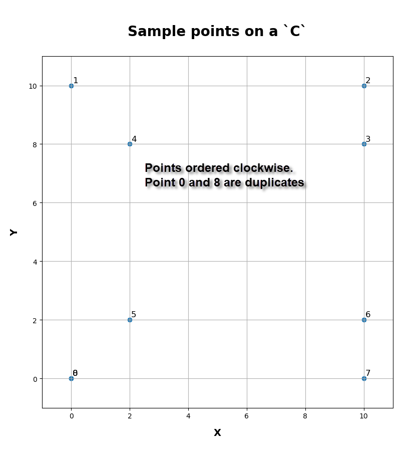
Start with a few points. The table and the graph below show what the arrangement is.

How was the table generated from the coordinates?

Every sequence needs an Id field, some x and y coordinates. The rest of the columns were calculated.

I will exclude the id column from the example, since all the other fields are decimal numbers.

Make an empty array to hold the results
Add the x and y coordinates (xs, ys)
Calculate the sequential differences in the coordinates (dx, dy)
Determine the segment lengths between the points (leng)
Calculate the cumulative length of the path formed by the points
Magic happens....

Sample Data Points...
id xs ys dx dy leng cumleng steps deltaX deltaY ---------------------------------------------------------------------------- 000 0.00 0.00 0.00 0.00 0.00 0.00 0.00 0.00 0.00 001 0.00 10.00 0.00 10.00 10.00 10.00 2.50 0.00 4.00 002 10.00 10.00 10.00 0.00 10.00 20.00 2.50 4.00 0.00 003 10.00 8.00 0.00 -2.00 2.00 22.00 0.50 0.00 -4.00 004 2.00 8.00 -8.00 0.00 8.00 30.00 2.00 -4.00 0.00 005 2.00 2.00 0.00 -6.00 6.00 36.00 1.50 0.00 -4.00 006 10.00 2.00 8.00 0.00 8.00 44.00 2.00 4.00 0.00 007 10.00 0.00 0.00 -2.00 2.00 46.00 0.50 0.00 -4.00 008 0.00 0.00 -10.00 0.00 10.00 56.00 2.50 -4.00 0.00

# ---- Procedure... start with an array 'a' a.shape # (9, 2) the input array, it has 9 rows and 2 columns (ie x, y) z = np.zeros((a.shape[0],9)) # make the empty array z[:, :2] = a # xys : x, y coordinates z[1:, 2:4] = dxdy = z[1:, :2] - z[:-1, :2] # sequential differences z[1:, 4] = np.sqrt(np.einsum('ij,ij->i', dxdy, dxdy)) # calculate distance z[:, 5] = np.cumsum(z[:,4]) # cumulative distance‍‍‍‍‍‍‍‍‍‍‍‍‍‍‍‍‍‍‍‍‍‍‍‍‍‍‍‍‍‍‍‍‍‍‍‍‍‍‍‍‍‍‍‍‍‍‍‍‍‍‍‍‍‍‍‍‍‍‍

The code so far

Start with a basic input of 9 points consisting of x and y values... it has a 'shape' property reflecting this.
Make a 'container' to hold our results in line 5... we will call it 'z'. To facilitate this, I made a numpy array filled with zeros. I would show it, but it is just an array with 9 rows ('a' is the points, and there are 9 of them) and 9 columns.
The 6th line fills columns 0 and 1 with the values in 'a'... in other words, the x and y coordinates
Stick with me... the 7th line fills in rows 1 to the end with two columns of data representing the sequential differences in the coordinates. z[1: .... means from the first row on, … 2:4] … means fill the 2nd and 3rd column (aka, the 'from, upto but not including' syntax)
Calculate the segment distances/lengths. I use einsum (Einstein summation). Its a long story, I have blogged about it elsewhere. Trust me it is fast and works with in multiple dimension and allows you way more tools other than distance calculations
Line 9 just does a cumulative summation of the distances.

What to do now?

Lots of things.

Basic geometric operations

shift, rotate, scale, skew

Derived geometric properties

interpoint distance (done), angles/directions/bearing, bounding boxes and way more

More later

But today, lets

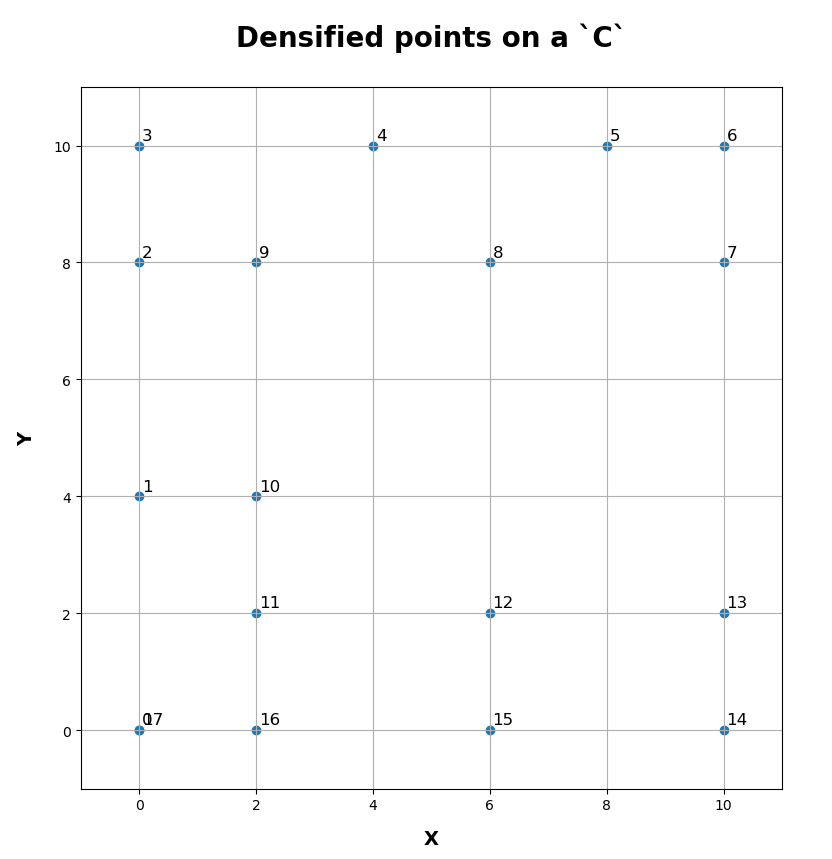
Densify the points

To add to the basic code, we are going to take a leap

The 7th column in the table above was labelled 'steps'. That columns was derived because I wanted to 'densify' the number of points between the input points. In this example, we will use a 'dist' of 4 units. This is line 1 below.

The 8th and 9th column need some explaining. I slipped that calculation in line 7 in the initial code.... dxdy

Between the first 2 points (0,0) and (0, 10), there is a 10 unit distance. Divide that by 4 and the first densification will have 2.5 steps in distance terms. In coordinate terms, we have a vertical line (right? check! so you understand). Out increment is obviously not going to be the same in the X and Y direction is it? The X coordinate will increment by 0 and the Y coordinate will increment by 4 (look at the 2nd row deltaX, deltaY columns). This calculation is done in line 2 below.

Densify by distance

z[1:, 6] = steps = z[1:, 4] / dist           # steps to create
z[1:, 7:] = deltas = dxdy/(steps.reshape(-1, 1))‍‍‍‍
#
# ---- above, calculating the steps and densification
# ---- below, for later... calculating the new points
#
N = len(a) - 1  # number of segments
pnts = np.empty((N,), dtype='O')
for i in range(N):              # cycle through the segments and make
    num = np.arange(steps[i])   # the new points
    pnts[i] = np.array((num, num)).T * deltas[i] + a[i]
a0 = a[-1].reshape(1,-1)
final = np.concatenate((*pnts, a0), axis=0)‍‍‍‍‍‍‍‍‍‍‍‍‍‍‍‍‍‍‍‍‍‍‍‍‍‍‍‍‍‍‍‍‍‍‍‍‍‍‍‍‍‍‍‍‍‍‍‍‍‍‍‍‍‍‍‍‍‍‍‍‍‍‍‍‍

So what does this produce? Out focus now turns to lines 7-13 above.

Sadly, we will be constructing arrays with 'jagged' shapes, object arrays, like geometry objects that don't have the same number of shapes, points or parts. (more in another blog). Basically line 8 above creates the container to save the results. Each 'row' can contain an indeterminate number of objects and each row's objects need not be the same length.

Line 10, produces the number of steps from our previous calculation. the np.arange function will truncate the decimal portion resulting in integer steps (ie steps = 2.5 results in

np.arange(2.5) # ---- array([0., 1., 2.])

Line 11 produces the points. Essentially line 11 is nothing more than the equation to calculate points along a line given a point and the line slope (or equivalent)

The zero in our arange, will be used to reproduce the first point, the 1 will be used to determine the position of the point 4 units up the Y axis and the 2 will be for the point up 8 units. That is.... (0, 0), (0, 4), and (0, 8). The last point between (0, 0) and (0, 10) will be created during the next sequence.

The points look like the following.

First sequence	2nd	3rd	4th ... and so on
step (0) ...points [[0. 0.] [0. 4.] [0. 8.]]	step (1) ...points [[ 0. 10.] [ 4. 10.] [ 8. 10.]]	step (2) ...points [[10. 10.]]	step (3) ...points [[10. 8.] [ 6. 8.]]

The first 4 sequences show how the points are produced.

We have already established that first sequence should produce 3 point, including the start point, two intermediate points but excluding the last.

The 2nd sequence is similar, and the end point of the first sequence is also the first point of the second.

The 3rd sequence... it is too short for any intervening points (have a look, it has a length/distance of 2), so only the first point is produced.

... carry on if you need it using the following.

Produce your own results
`for i, pnt in enumerate(pnts): print("\nstep ({}) ...points\n{}".format(i, pnt))‍‍‍‍‍‍‍‍`

The final result is a sequence of points which represent the densified input pattern.

Points ... translated/rotated for viewing.
final.T array([[ 0., 0., 0., 0., 4., 8., 10., 10., 6., 2., 2., 2., 6., 10., 10., 6., 2., 0.], [ 0., 4., 8., 10., 10., 10., 10., 8., 8., 8., 4., 2., 2., 2., 0., 0., 0., 0.]])

Pretty much it.

Next steps... just produce the points, produce a polyline using the points, subdivide the points into segments of fixed and/or variable lengths, add a Z dimension to the results... whatever..