- Home
- :
- All Communities
- :
- Products
- :
- ArcGIS Spatial Analyst
- :
- ArcGIS Spatial Analyst Blog
- :
- Creating accumulative cost surfaces using directio...
Creating accumulative cost surfaces using directional data
- Subscribe to RSS Feed
- Mark as New
- Mark as Read
- Bookmark
- Subscribe
- Printer Friendly Page
The following question was recently posted to GeoNet:
“I want to add wind direction and strength to a cost distance surface. How do I create a raster surface which incorporates these two factors…?“
In this blog post, the spatial analyst team responds to this user’s question.
The Path Distance tool in the Spatial Analyst toolbox can do part of this. It can be used to create an accumulative cost surface from costs that are determined by the direction of the wind. Unfortunately, Esri doesn’t yet have a way to make cost of motion vary based on both the direction and speed of the wind.
Also, when using Path Distance, it is extremely important to know in advance whether you intend to move from source cells to other cells, or vice versa. You will see that changing this intent changes the result dramatically.
If you decide to use Path Distance to incorporate only wind direction into your accumulative cost surface, here is what we recommend:
You can encode wind direction azimuths (clockwise 0-360 from north, both 0 and 360 are treated as “north”) in the input horizontal raster. In figure 1 below, a 10 x 10 horizontal raster is shown. It has a constant cell value of 90 and represents wind blowing to the east with some uniform speed over the study area.
You should not use wind speed as the friction cost surface, because that cost is paid regardless of which direction you travel through a cell. In fact, Path Distance doesn’t need a cost friction surface at all (nor do the other Path Distance tools: allocation, backlink).
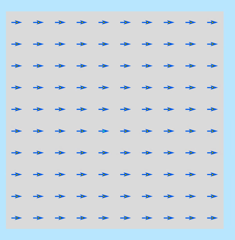
Figure 1-A 10 x 10 horizontal direction raster used as input to Path Distance. Each cell has a value of 90 (wind blowing from west to east). Cell centers are shown in yellow, along with a vector field renderer (blue arrows).
Case 1: Motion from source
Let’s first assume that:
- You are sitting on the single source point (the selected blue point in the center of the raster in figure 2).
- That its easiest to move with the wind and impossible to move either against it or at right angles to it.
- That you want to calculate accumulated cost from your source cell to every other cell in the study area.
For this case, you could use a horizontal_factor parameter value of Horizontal Forward Function AND (this is important) a source_direction parameter value of “FROM_SOURCE”. The result is shown in figure 2. You can see that your accumulated cost surface is only defined in areas that can be reached travelling with (or somewhat with) the wind.
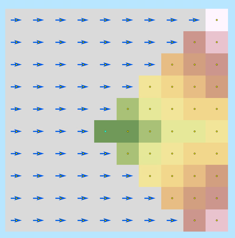
Figure 2- The results of using Path Distance with the horizontal raster from figure 1 and the horizontal forward function. The single source is the selected point in the center and we want to know how expensive it is to reach other cells in the study area. The accumulated cost surface shows that we are only allowed to move with the wind, and its easiest to move directly east. For this result, we use the horizontal forward function AND a source_direction parameter value of motion from source.
Lets go into a bit of detail on how Path Distance turns wind direction into a travel cost (also called a weight). We zoom in on the single source cell and its 8 neighbors:
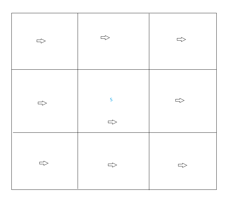
Figure 3 - Detail of source cell (marked with an S) and its 8 neighbors. Each cell has a wind direction.
From that source, we can move in 8 directions to reach a neighbor cell and we need to figure out what the step cost for that move will be.
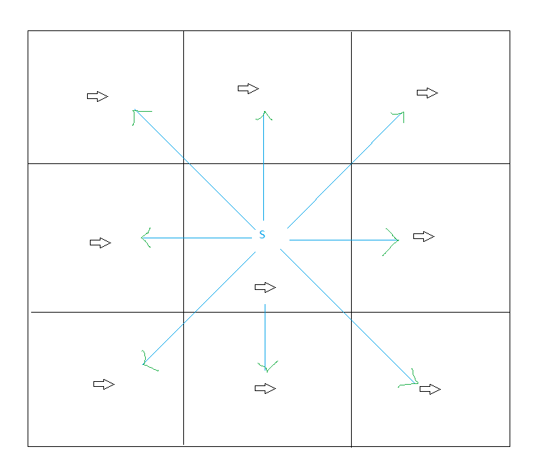
Figure 4 - You can move 8 ways from the source cell to its neighbors. Each choice makes a different angle relative to each cell's wind direction.
In our case, the only thing that affects the step cost is wind direction. Each of those 8 step directions makes some angle with the preferred moving direction, which in this case is the wind direction.
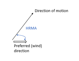
HRMA calculation
We call this angle the horizontal relative moving angle (HRMA) because it is your direction of motion relative to an azimuth value stored in your horizontal raster. Each horizontal factor function turns this HRMA into a weight. In this case, we’ve used the Horizontal Forward Function. See this help topic for more details on HRMA.
The HRMA and horizontal factor function are evaluated twice for each of the 8 possible steps: once for the wind direction at the source cell and once for the direction at the neighbor cell. The two results are then averaged to get the horizontal weight to be used when calculating the cost of a step into the neighbor cell.
Case 2: Motion To Source
Now let’s assume that the single source point represents a location that you want to reach from other points in the study area. In this case, all inputs to Path Distance remain the same, except you now choose a source _direction parameter value of “TO_SOURCE”. Figure 5 shows the result. As you can see, the results are very different.
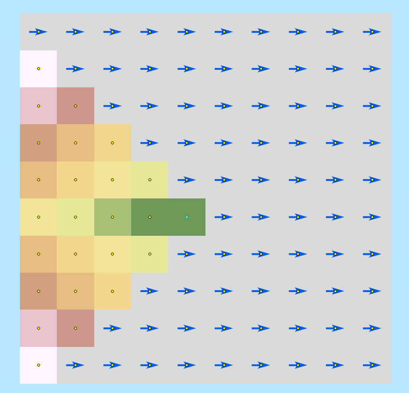
Figure 5 -The result of using Path Distance to find accumulated cost of travelling to the single source point from other cells in the study area: source_direction is set to “ motion to source”. All other inputs are the same as for figure 2.
Why are these results so different? In both cases, the accumulative cost surface is grown outward starting from the source and visiting all other cells; but in the TO_SOURCE case, the calculation of the HRMA is different, so the output of the horizontal factor function applied to that HRMA will also be different. In the TO_SOURCE case the HRMA is the geometric supplement of the HRMA calculated in the FROM_SOURCE case, as shown in figure 6.
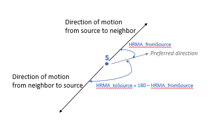
HRMA value changes based on direction of motion
To summarize:
Path distance can adjust the cost of motion through a cell based on input data that describes, for each cell, the easiest direction to move through the cell. This calculation can produce very different results, based on whether you want to move from a source to other cells, or from other cells back to the source.
We haven’t explicitly talked about the vertical raster and vertical factor functions, but the reasoning process is basically the same as described above. However, instead of accounting for horizontal influences, the vertical factor determines the cost to overcome the changes in elevations (the slopes) between the cells.
The original blog content has been written by James TenBrink and Kevin Johnston and is available here: https://www.esri.com/arcgis-blog/products/arcgis-pro/analytics/creating-accumulative-cost-surfaces-u...
James TenBrink is a senior software engineer in the raster analysis group at esri. He has a Bachelor of Science degree in Computer Science from Hope College in Holland, Michigan, and a Master of Science degree in Computer Science from Rensselaer Polytechnic Institute in Troy, New York. He has been with esri 28 years and has had an office in almost every building, on almost every floor, of the esri campus.
Kevin Johnston has been a Product Engineer on the Spatial Analyst development team for over 29 years. He has degrees in Landscape Architect from Harvard and in environmental modeling from Yale. At Esri, Kevin’s current focus is developing suitability and connectivity tools. He hopes the tools that he works on can help users make more informed decisions.
You must be a registered user to add a comment. If you've already registered, sign in. Otherwise, register and sign in.