
foto por Kevin Jarrett no Unsplash
Atualização 17/03/2025: Um analisador JSON de exemplo para python pode ser encontrado anexado a este artigo. Você também pode encontrar um analisador de exemplo construído usando o ArcGIS Pro SDK no repositório GitHub do ArcGIS Developer & Technology Summit 2025.
Você já quis construir sua própria análise usando o modelo de conectividade da ArcGIS Utility Network, mas teve dificuldades para analisar os arquivos JSON que a ferramenta Export Subnetwork ou Trace produz? Talvez você tenha um produto de análise de rede que deseja integrar com a utility network?
Python pode ser seu trunfo ao construir um analisador poderoso que transforma seu JSON em um grafo utilizável, e este artigo mostrará como. Com o grafo em mãos, você terá a liberdade de conduzir sua própria análise de rede ou usá-lo para preencher outra ferramenta de análise de sua escolha.
Este artigo tem a intenção de complementar o artigo Journey to the Utility Network: Network Integrations publicado em junho passado. Para aproveitar ao máximo os exemplos deste artigo, recomendo que você leia esse artigo primeiro e tenha uma familiaridade básica com Python, bem como os conceitos básicos e terminologia da ArcGIS Utility Network. A Referência Python do ArcGIS Pro e a página Utility Network Vocabulary são bons recursos para começar caso precise de ajuda.
Certifique-se também de baixar o JSON de exemplo e o analisador anexados a este artigo para que você possa acompanhar. Este JSON neste artigo é do modelo Water Utility Network, mas você verá que os arquivos de exemplo anexados podem ser adaptados para diferentes modelos de dados ou versões. O artigo é escrito para seguir a estrutura do script anexado, mas você pode usar a lista abaixo para ver quais elementos JSON no arquivo são discutidos neste artigo.
- Mapeamento da Fonte
- Referência Espacial
- Features
- Conectividade
- Associações
O arquivo JSON que usaremos neste exemplo inclui os três principais tipos de resultado do Export Subnetwork: features, conectividade e associações. Escolhi incluir geometrias e descrições de domínio nesta exportação para tornar o arquivo mais fácil de entender e analisar, mas essas opções aumentarão visivelmente o tamanho do arquivo JSON resultante, então se sua aplicação não requer essa informação, você deve deixar essas opções desmarcadas.
Carregando o arquivo
A primeira coisa que devemos fazer para analisar o arquivo é carregar o arquivo JSON do disco para a memória. Embora pudéssemos ler o conteúdo do arquivo diretamente na memória, é melhor usar uma biblioteca de análise JSON como UJSON para ler e analisar o arquivo para nós. Fazer isso nos permitirá interagir com o JSON no arquivo usando estruturas normais de dados Python sem precisar se preocupar em como analisar todas as chaves e aspas no arquivo. Você pode ver isso acontecendo no início do método ParseJsonExport.
with open(json_path, "r") as json_file:
    json_content = ujson.load(json_file)
del json_file
Uma vez que carregamos o arquivo e permitimos que a biblioteca UJSON o analise, podemos então interagir com seu conteúdo como faríamos com qualquer outro objeto Python. A maioria dos elementos no arquivo JSON são representados usando dicionários ou arrays. Você pode ver uma visão geral da estrutura do arquivo, conforme representado em JSON abaixo:
{
    "connectivity": [
        {  },
    ],
    "featureElements": [
        {  },
    ],
    "associations": [
        {  },
    ],
    "sourceMapping": {  },
    "spatialReference": {  }
}
Para mais informações sobre como controlar a saída do arquivo para incluir mais ou menos informações, consulte o artigo Utility Network Integrations article referenciado acima. Por enquanto, vamos continuar analisando como o script de análise utiliza cada um desses elementos.
Mapeamento da Fonte
O elemento “sourceMapping” fornece um dicionário que traduz os nomes das camadas para todas as fontes da rede na sua utility network para um identificador interno (network source id) mantido pela utility network. Isso é importante porque o resto do arquivo JSON referencia features pelo network source id, então se você quiser saber se uma feature é um dispositivo, linha ou estrutura e escolheu não incluir descrições na sua exportação, precisará consultar essa tradução.
"sourceMapping": {
        "1": "UN_134_Associations",
        "2": "UN_134_SystemJunctions",
        "3": "",
        "4": "StructureJunction",
        "6": "StructureBoundary",
        "7": "StructureJunctionObject",
        "5": "StructureLine",
        "8": "StructureEdgeObject",
        "9": "WaterDevice",
        "11": "WaterAssembly",
        "12": "WaterJunction",
        "14": "WaterJunctionObject",
        "10": "WaterLine",
        "13": "WaterSubnetLine",
        "15": "WaterEdgeObject"
    },
Como o elemento source mapping é um dicionário, aproveitar seu poder é simples. Uma vez que temos uma referência a este elemento, podemos facilmente utilizá-lo para traduzir IDs das fontes da rede sempre que necessário. A exportação incluída neste exemplo já inclui descrições para todas as nossas fontes da rede; no entanto, você pode ver que o analisador ainda está usando os mapeamentos das fontes para traduzir informações nos casos em que você cria uma exportação que não inclui descrições de domínio.
feature_values['networkSourceName'] = source_mapping.get(element['networkSourceId'], "Unknown")
Agora que você viu como usamos mapeamentos das fontes para processar elementos, vamos ver como podemos usar o elemento spatial reference para ajudar a criar uma geometria.
Referência Espacial
O elemento “spatialReference” descreve a referência espacial da utility network da qual a exportação foi feita e só precisa ser considerado ao fazer uso das geometrias incluídas no arquivo. O primeiro passo que precisamos dar é transformar o elemento spatial reference em JSON em um objeto spatial reference usando ArcPy.
spatial_reference_element = json_content.get("spatialReference", None)
if spatial_reference_element is not None:
        spatial_reference = arcpy.SpatialReference(spatial_reference_element["wkid"])
arcpy.CreateFeatureclass_management(output_gdb,"trace_point","POINT",spatial_reference=spatial_reference)
arcpy.CreateFeatureclass_management(output_gdb,"trace_line","POINT",spatial_reference=spatial_reference)
Note, depending on your release and which method you use to export your JSON the resulting JSON file may not have a spatial reference element. If this is the case, you can always use the spatial reference of the utility network dataset itself using the following code:
un_description = arcpy.Describe(utility_network)
spatial_reference = un_description.spatialReference
Populating these feature classes requires us to parse the features element of the JSON file to extract geometry and attribute information. Conveniently enough, that’s the next thing that our script does.
Features
The “featuresElements” element in the JSON file contains the attribute information for all the features included in your subnetwork or trace. The biggest challenge when interpreting this section of the file is to remember that the network’s representation of your features is more granular than the representation you see in the map. To illustrate, let’s look at an example.
In your map, a junction or single-terminal device is represented as a point feature. In the JSON file, you will find that it corresponds to a single element.

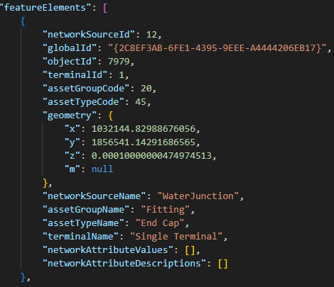
Things get more interesting when you look at a device that has two (or more) terminals. In the map this will appear as a single feature, but in the export, it is represented as multiple elements. The export treats each terminal and terminal path as a separate feature.


This may seem a little unusual at first glance, but its importance is understood once you start comparing the contents of this file with the connectivity portions of the JSON file which reference the individual terminal and edges to establish connectivity. To uniquely identify each point element in the JSON file we could use the network source id, object id, and terminal id of the feature (which would match the connectivity). However, you will notice that in our parser we have chosen to uniquely identify each feature using just the network source id and object id of each feature. This reduces redundancy and means that to look up attribute information you need only a network source id and object id.
feature_key = f"{element['networkSourceId']}${element['objectId']}"
The next difference you will note is in how line features are represented. This is because, in the utility network, each line feature is represented by one or more edge elements. When a line has midspan connectivity then the network uses multiple edge elements to represent each of the sections of the line. You can see this in the example below where the line feature in our geodatabase has two feature elements in the file, each representing a different segment of the line.


To uniquely identify the attributes of each feature, it is sufficient to consider the network source id and object id of the feature. However, to consolidate the geometries for the feature we must consider the from position and to position of each edge because each JSON element represents a subset of the overall line’s geometry. Using the example from above we can see that the first segment accounts for 59% of the shape’s length, with the second segment accounting for the remaining 41%.
Similar to how we handled point features, our parser has chosen to consolidate all the attributes for edge elements into a single feature using the network source id and object id. For the geometries however, we are storing the “from position” of the JSON element along with the coordinates of the line so we can consolidate the geometries from multiple features into a single geometry.
Você pode ver a diferença entre como estamos armazenando geometrias para feições de ponto e linha no trecho abaixo.
para chave, valor em element.items():
    se chave == "geometry":
        geometry_element = valor
        se "x" em geometry_element:
            # Criar um ponto
            geometries[feature_key] = arcpy.Point(geometry_element["x"],geometry_element["y"],geometry_element["z"],geometry_element["m"])
        elif "fromPosition" em element:
            # Anexar a geometria do segmento de linha, junto com a posição ao longo da porcentagem
            # Usamos isso para unir todos os segmentos de linha depois
            other_geometries = geometries.get(feature_key, [])
            other_geometries.append([element["fromPosition"], geometry_element])
            geometries[feature_key] = other_geometries
Embora não discutamos a criação de geometrias neste artigo, você pode olhar o método CreateGeometries na ferramenta anexada para um exemplo de como preencher uma classe de feição com as geometrias usando esta exportação. Se sua exportação não precisar usar informações de geometria, você pode simplificar seu parser e reduzir muito o tamanho do arquivo simplesmente excluindo geometrias da sua saída e fazendo seu parser ignorá-las.
Conectividade
O elemento "connectivity" no arquivo JSON é um grafo não direcionado que é uma coleção de nós e arestas. Cada elemento de conexão descreve uma aresta que conecta dois nós onde os atributos from/to do elemento JSON referem-se a um nó e os atributos via do elemento JSON referenciam a aresta.

Conectividade entre elementos
O script incluído mostra como conseguir isso usando o método ProcessConnectivity. Este método analisa os elementos de conectividade em seus componentes separados from/via/to usando duas abordagens diferentes.
- Os elementos from e to são identificados exclusivamente por seu id da fonte da rede, id do objeto e seu id terminal.
- Os elementos via são então identificados exclusivamente pelo id da fonte da rede, id do objeto, posição "from" e posição "to".
para element em connectivity_element:
    from_key = f"{element['fromNetworkSourceId']}${element['fromObjectId']}${element['fromTerminalId']}"
    to_key = f"{element['toNetworkSourceId']}${element['toObjectId']}${element['toTerminalId']}"
    via_key = f"{element['viaNetworkSourceId']}${element['viaObjectId']}${element['viaPositionFrom']}${element['viaPositionTo']}"
Uma vez que todos os elementos from/via/to foram analisados, podemos então usar essa informação para criar uma lista de adjacência. No caso deste parser, tratamos cada elemento from/via/to como seu próprio objeto e armazenamos as conexões entre cada um deles. Esta estrutura é bem adequada para análise usando um algoritmo de travessia de rede, ou para análise usando bibliotecas Python como networkx.
# Armazenar a conectividade
from_connections = connectivity.get(from_key, [])
from_connections.append(via_key)

via_connections = connectivity.get(via_key, [])
via_connections.append(to_key)

# Se a conexão via for uma associação de conectividade, precisamos adicionar arestas para ambos os lados
# Já que não permitimos especificar direção digitalizada em uma associação
se element["viaNetworkSourceId"] == 1:
    to_connections = connectivity.get(to_key, [])
    to_connections.append(via_key)
    connectivity[to_key] = to_connections

    via_connections.append(from_key)

connectivity[from_key] = from_connections
connectivity[via_key] = via_connections
É importante lembrar que a conectividade neste arquivo JSON não possui direcionalidade, fluxo ou informação sobre atravessabilidade. De forma mais simples, a direcionalidade implícita pela nomeação das informações from, via e to não representa fluxo real dentro da rede de utilidades, ao invés disso, representa a ordem dos vértices em uma linha ou a origem/destino da associação (nenhum dos quais indicam fluxo). O fluxo verdadeiro da rede de utilidades é calculado usando fontes ou sumidouros quando o traço é realizado e atualmente não é exportado no JSON. Você pode ver um exemplo disso no gráfico abaixo onde algumas das arestas parecem estar "invertidas". Nesta área, o fluxo real da água está fluindo de uma área de alta pressão à direita para uma área de baixa pressão à esquerda, entretanto, a direção digitalizada das linhas no mapa e JSON mostra o extremo "from" das linhas vindo da esquerda para a direita.

O elemento connectivity inclui geometrias para feições de maneira semelhante ao elemento features, o que significa que cada elemento espacial from/via/to incluirá sua geometria e o elemento edge da geometria pode corresponder a um subconjunto da geometria geral para a aresta se a feição edge contiver múltiplos elementos edge como visto abaixo.
Agora que cobrimos como processar features e conectividade, a última peça restante do quebra-cabeça é o elemento "associations".
{
    "viaNetworkSourceId": 10,
    "viaGlobalId": "{29C0B239-9AC0-4E76-9E5A-A912D46CF267}",
    "viaObjectId": 22258,
    "viaPositionFrom": 0.59016310696272389,
    "viaPositionTo": 1,
    "viaGeometry": {
        "hasZ": true,
        "hasM": true,
        "paths": [
            [
                [
                    1032056.63583742827,
                    1857139.22013278306,
                    0.00010000000474974513,
                    null
                ],
                [
                    1032024.145088762,
                    1857269.34913761169,
                    0.00010000000474974513,
                    null
                ]
            ]
        ]
    },
    "fromNetworkSourceId": 12,
    "fromGlobalId": "{6F988B32-CA53-4DE2-AA77-A79544386D3F}",
    "fromObjectId": 7271,
    "fromTerminalId": 1,
    "fromGeometry": {
        "x": 1032056.63583742827,
        "y": 1857139.22013278306,
        "z": 0.00010000000474974513,
        "m": null
    },
    "toNetworkSourceId": 12,
    "toGlobalId": "{4F36DEA2-656D-468D-B1F9-30849B04FC20}",
    "toObjectId": 7723,
    "toTerminalId": 1,
    "toGeometry": {
        "x": 1032024.145088762,
        "y": 1857269.34913761169,
        "z": 0.00010000000474974513,
        "m": null
    }
},
Associations
The “associations” JSON element is very similar to the “connectivity” element JSON in structure with the exception that each element consists of only a “from” and “to” element. Additionally, the utility network models associations at the feature level, so when cross-referencing associations to the features element you only need to consider the network source id and the global id of the “from” and “to” feature.
{
    "associationType": "containment",
    "fromNetworkSourceId": 6,
    "fromGlobalId": "{E4693E2A-441D-404F-871F-4D4C5E6AE20A}",
    "fromTerminalId": 1,
    "toNetworkSourceId": 9,
    "toGlobalId": "{FC1540AA-5965-4BDD-B207-F6AD0B40B5BE}",
    "toTerminalId": 1,
    "fromNetworkSourceName": "StructureBoundary",
    "fromTerminalName": "Single Terminal",
    "toNetworkSourceName": "WaterDevice",
    "toTerminalName": "Single Terminal"
},
By parsing the JSON this way, you can filter out what appear as duplicate associations. Doing this before outputting your results will make it easier to interpret your results as well as reduce the size of any files you output.
{
    "associationType": "containment",
    "fromNetworkSourceId": 5,
    "fromGlobalId": "{8F686F75-3E07-4EFA-BAA4-EAE03F40D93F}",
    "fromTerminalId": -1,
    "toNetworkSourceId": 10,
    "toGlobalId": "{92D69B81-FF17-4C5A-85CB-0733AFE8F02A}",
    "toTerminalId": -1,
    "fromNetworkSourceName": "StructureLine",
    "fromTerminalName": "",
    "toNetworkSourceName": "WaterLine",
    "toTerminalName": ""
},
… association repeats multiple times …
{
    "associationType": "containment",
    "fromNetworkSourceId": 5,
    "fromGlobalId": "{8F686F75-3E07-4EFA-BAA4-EAE03F40D93F}",
    "fromTerminalId": -1,
    "toNetworkSourceId": 10,
    "toGlobalId": "{92D69B81-FF17-4C5A-85CB-0733AFE8F02A}",
    "toTerminalId": -1,
    "fromNetworkSourceName": "StructureLine",
    "fromTerminalName": "",
    "toNetworkSourceName": "WaterLine",
    "toTerminalName": ""
},
Note that because we are referencing associations by network source id and global id, while referencing other features by their network source id and object id we will need to do some translation when comparing the different datasets. In this example, the use of the object id was a deliberate choice to make it simpler to select and interact with the geodatabase, but for other applications it may be easier to not use object id for any comparisons and just use the global id.
Conclusion
Now that you have read this article you are equipped with a better understanding of interpreting and parsing the features, connectivity, and associations elements in JSON files produced by the utility network. To inspire you further, attached to this article is a sample Python tool that demonstrates how these techniques can be used to craft your own custom analysis. Happy parsing!