
foto door Kevin Jarrett op Unsplash
Update 17-3-2025: Een voorbeeld van een JSON-parser voor python is bij dit artikel gevoegd. Je kunt ook een voorbeeldparser vinden die is gebouwd met de ArcGIS Pro SDK in de GitHub-repository van de 2025 ArcGIS Developer & Technology Summit.
Heb je ooit je eigen analyse willen bouwen met het connectiviteitsmodel van het ArcGIS Utility Network, maar moeite gehad met het parseren van de JSON-bestanden die het Export Subnetwork of Trace-gereedschap produceert? Misschien heb je een netwerkanalyseproduct dat je wilt integreren met het utility network?
Python kan je geheime wapen zijn bij het bouwen van een krachtige parser die je JSON omzet in een bruikbare grafiek, en dit artikel laat je zien hoe. Met de grafiek in handen heb je de vrijheid om je eigen netwerkanalyses uit te voeren of deze te gebruiken om een ander analysetool naar keuze te vullen.
Dit artikel is bedoeld als aanvulling op het Journey to the Utility Network: Network Integrations-artikel dat afgelopen juni is gepubliceerd. Om het meeste uit de voorbeelden in dit artikel te halen, raad ik aan dat je dat artikel eerst leest en een basiskennis hebt van Python evenals de basisconcepten en terminologie van het ArcGIS Utility Network. De ArcGIS Pro Python Reference en Utility Network Vocabulary-pagina zijn goede bronnen om mee te beginnen als je hulp nodig hebt.
Zorg er ook voor dat je de voorbeeld-JSON en parser downloadt die bij dit artikel zijn gevoegd zodat je kunt meedoen. De JSON in dit artikel komt uit het Water Utility Network-model, maar je zult merken dat de bijgevoegde voorbeeldbestanden kunnen worden aangepast aan verschillende datamodellen of releases. Het artikel is geschreven om de structuur van het bijgevoegde script te volgen, maar je kunt onderstaande lijst gebruiken om te zien welke JSON-elementen in het bestand in dit artikel worden besproken.
- Bronmapping
- Ruimtelijke referentie
- Features
- Connectiviteit
- Associaties
Het JSON-bestand dat we in dit voorbeeld gebruiken bevat de drie belangrijkste resultaattypes van Export Subnetwork: features, connectiviteit en associaties. Ik heb ervoor gekozen om geometrieën en domeinbeschrijvingen in deze export op te nemen om het bestand gemakkelijker te begrijpen en te parseren, maar deze opties vergroten merkbaar de grootte van het resulterende JSON-bestand, dus als je toepassing deze informatie niet vereist, moet je deze opties uitvinken.
Bestand laden
Het eerste wat we moeten doen om het bestand te parseren is het JSON-bestand vanaf schijf in het geheugen laden. Hoewel we de inhoud van het bestand direct in het geheugen kunnen lezen, is het beter om een JSON-parserbibliotheek zoals UJSON te gebruiken om het bestand voor ons te lezen en te parseren. Dit stelt ons in staat om met de JSON in het bestand te werken met normale Python-datastructuren zonder ons zorgen te maken over hoe we alle accolades en aanhalingstekens in het bestand moeten parsen. Je ziet dit gebeuren aan het begin van de ParseJsonExport-methode.
with open(json_path, "r") as json_file:
    json_content = ujson.load(json_file)
del json_file
Zodra we het bestand hebben geladen en de UJSON-bibliotheek het heeft geparsed, kunnen we vervolgens met de inhoud ervan werken zoals met elk ander Python-object. De meeste elementen in het JSON-bestand worden weergegeven met behulp van dictionaries of arrays. Hieronder zie je een overzicht van de bestandsstructuur zoals weergegeven in JSON:
{
    "connectivity": [
        {  },
    ],
    "featureElements": [
        {  },
    ],
    "associations": [
        {  },
    ],
    "sourceMapping": {  },
    "spatialReference": {  }
}
Voor meer informatie over hoe je de uitvoer van het bestand kunt regelen om meer of minder informatie op te nemen, verwijzen we naar het hierboven genoemde Utility Network Integrations-artikel referenced above. For now, let’s continue analyzing how the parsing script makes use of each of these elements.
Source Mapping
The “sourceMapping” element provides a dictionary that translates the layer names for all the network sources in your utility network to an internal identifier (network source id) maintained by the utility network. This is important because the rest of the JSON file references features by their network source id, so if you want to know whether a feature is a device, line, or structure and you chose not to include descriptions in your export you will need to refer to this translation.
"sourceMapping": {
        "1": "UN_134_Associations",
        "2": "UN_134_SystemJunctions",
        "3": "",
        "4": "StructureJunction",
        "6": "StructureBoundary",
        "7": "StructureJunctionObject",
        "5": "StructureLine",
        "8": "StructureEdgeObject",
        "9": "WaterDevice",
        "11": "WaterAssembly",
        "12": "WaterJunction",
        "14": "WaterJunctionObject",
        "10": "WaterLine",
        "13": "WaterSubnetLine",
        "15": "WaterEdgeObject"
    },
As the source mapping element is a dictionary, harnessing its power is simple. Once we have a reference to this element, we can easily utilize it to translate network source IDs whenever the need arises. The export included in this example already includes descriptions for all our network sources, however, you can see that the parser is still using the source mappings to translate information in cases where you create an export that doesn’t include domain descriptions.
feature_values['networkSourceName'] = source_mapping.get(element['networkSourceId'], "Unknown")
Now that you’ve seen how we use source mappings to process elements, let’s look at how we can use the spatial reference element to help create a geometry.
Spatial Reference
The “spatialReference” element describes the spatial reference of the utility network from which the export was taken and only needs to be considered when making use of the geometries included in the file. The first step we need to take is to turn the spatial reference element in JSON into a spatial reference object using ArcPy.
spatial_reference_element = json_content.get("spatialReference", None)
if spatial_reference_element is not None:
        spatial_reference = arcpy.SpatialReference(spatial_reference_element["wkid"])
If you want to visualize your results the spatial reference must be included when creating any geometries or datasets or when translating the geometries to another coordinate system. You can see an example of this below:
arcpy.CreateFeatureclass_management(output_gdb,"trace_point","POINT",spatial_reference=spatial_reference)
arcpy.CreateFeatureclass_management(output_gdb,"trace_line","POINT",spatial_reference=spatial_reference)
Note, depending on your release and which method you use to export your JSON the resulting JSON file may not have a spatial reference element. If this is the case, you can always use the spatial reference of the utility network dataset itself using the following code:
un_description = arcpy.Describe(utility_network)
spatial_reference = un_description.spatialReference
Populating these feature classes requires us to parse the features element of the JSON file to extract geometry and attribute information. Conveniently enough, that’s the next thing that our script does.
Features
The “featuresElements” element in the JSON file contains the attribute information for all the features included in your subnetwork or trace. The biggest challenge when interpreting this section of the file is to remember that the network’s representation of your features is more granular than the representation you see in the map. To illustrate, let’s look at an example.
In your map, a junction or single-terminal device is represented as a point feature. In the JSON file, you will find that it corresponds to a single element.

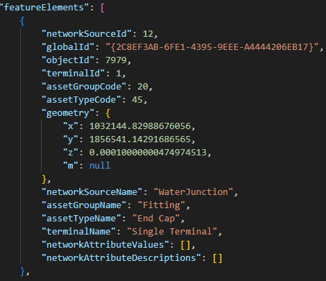
Things get more interesting when you look at a device that has two (or more) terminals. In the map this will appear as a single feature, but in the export, it is represented as multiple elements. The export treats each terminal and terminal path as a separate feature.


This may seem a little unusual at first glance, but its importance is understood once you start comparing the contents of this file with the connectivity portions of the JSON file which reference the individual terminal and edges to establish connectivity. To uniquely identify each point element in the JSON file we could use the network source id, object id, and terminal id of the feature (which would match the connectivity). However, you will notice that in our parser we have chosen to uniquely identify each feature using just the network source id and object id of each feature. This reduces redundancy and means that to look up attribute information you need only a network source id and object id.
feature_key = f"{element['networkSourceId']}${element['objectId']}"
The next difference you will note is in how line features are represented. This is because, in the utility network, each line feature is represented by one or more edge elements. When a line has midspan connectivity then the network uses multiple edge elements to represent each of the sections of the line. You can see this in the example below where the line feature in our geodatabase has two feature elements in the file, each representing a different segment of the line.


To uniquely identify the attributes of each feature, it is sufficient to consider the network source id and object id of the feature. However, to consolidate the geometries for the feature we must consider the from position and to position of each edge because each JSON element represents a subset of the overall line’s geometry. Using the example from above we can see that the first segment accounts for 59% of the shape’s length, with the second segment accounting for the remaining 41%.
Similar to how we handled point features, our parser has chosen to consolidate all the attributes for edge elements into a single feature using the network source id and object id. For the geometries however, we are storing the “from position” of the JSON element along with the coordinates of the line so we can consolidate the geometries from multiple features into a single geometry.
Je kunt het verschil zien tussen hoe we geometrieën opslaan voor punt- en lijnkenmerken in het onderstaande fragment.
voor sleutel, waarde in element.items():
    als sleutel == "geometry":
        geometry_element = waarde
        als "x" in geometry_element:
            # Maak een punt aan
            geometrieën[feature_key] = arcpy.Point(geometry_element["x"],geometry_element["y"],geometry_element["z"],geometry_element["m"])
        elif "fromPosition" in element:
            # Voeg de geometrie van het lijnsegment toe, samen met de positie langs het percentage
            # We gebruiken dit om later alle lijnsegmenten aan elkaar te koppelen
            andere_geometrieën = geometrieën.get(feature_key, [])
            andere_geometrieën.append([element["fromPosition"], geometry_element])
            geometrieën[feature_key] = andere_geometrieën
Hoewel we in dit artikel niet bespreken hoe je geometrieën maakt, kun je de CreateGeometries-methode in de bijgevoegde tool bekijken voor een voorbeeld van hoe je een feature class vult met de geometrieën met behulp van deze export. Als je export geen gebruik hoeft te maken van geometrie-informatie, kun je je parser vereenvoudigen en de bestandsgrootte aanzienlijk verkleinen door simpelweg geometrieën uit je output uit te sluiten en je parser ze te laten negeren.
Connectiviteit
Het "connectivity"-element in het JSON-bestand is een ongerichte graaf die bestaat uit knooppunten en verbindingen. Elk connectie-element beschrijft een verbinding die twee knooppunten verbindt waarbij de from/to-attributen van het JSON-element elk verwijzen naar een knooppunt en de via-attributen van het JSON-element verwijzen naar de verbinding.

Connectiviteit tussen elementen
Het bijgevoegde script laat zien hoe dit te bereiken met behulp van de ProcessConnectivity-methode. Deze methode analyseert de connectiviteitselementen in hun afzonderlijke from/via/to-componenten met behulp van twee verschillende benaderingen.
- De from- en to-elementen worden elk uniek geïdentificeerd door hun netwerkbron-id, object-id en hun terminal-id.
- De via-elementen worden vervolgens uniek geïdentificeerd door de netwerkbron-id, object-id, "from" positie en "to" positie.
voor element in connectivity_element:
    from_key = f"{element['fromNetworkSourceId']}${element['fromObjectId']}${element['fromTerminalId']}"
    to_key = f"{element['toNetworkSourceId']}${element['toObjectId']}${element['toTerminalId']}"
    via_key = f"{element['viaNetworkSourceId']}${element['viaObjectId']}${element['viaPositionFrom']}${element['viaPositionTo']}"
Zodra alle from/via/to-elementen zijn geparseerd, kunnen we deze informatie gebruiken om een adjacency-lijst te maken. In het geval van deze parser behandelen we elk from/via/to-element als een eigen object en slaan we de verbindingen tussen elk van hen op. Deze structuur is goed geschikt voor analyse met behulp van een netwerkdoorloopalgoritme, of voor analyse met Python-bibliotheken zoals networkx.
# Sla de connectiviteit op
from_connections = connectivity.get(from_key, [])
from_connections.append(via_key)

via_connections = connectivity.get(via_key, [])
via_connections.append(to_key)

# Als de via-verbinding een connectiviteitsassociatie is, moeten we randen aan beide zijden toevoegen
# Omdat we geen gedigitaliseerde richting op een associatie toestaan
als element["viaNetworkSourceId"] == 1:
    to_connections = connectivity.get(to_key, [])
    to_connections.append(via_key)
    connectivity[to_key] = to_connections

    via_connections.append(from_key)

connectivity[from_key] = from_connections
connectivity[via_key] = via_connections
Het is belangrijk om te onthouden dat de connectiviteit in dit JSON-bestand geen richting, stroom of informatie over begaanbaarheid bezit. Simpel gezegd vertegenwoordigt de richting die wordt geïmpliceerd door de naamgeving van from, via en to informatie niet de werkelijke stroom binnen het utility network; in plaats daarvan vertegenwoordigt het de volgorde van de vertices in een lijn of de oorsprong/bestemming van de associatie (geen van beide duidt op stroom). De werkelijke stroom van het utility network wordt berekend met behulp van bronnen of putten wanneer de trace wordt uitgevoerd en wordt momenteel niet uitgegeven in het JSON-bestand. Je kunt een voorbeeld hiervan zien in de onderstaande afbeelding waar sommige verbindingen lijken te zijn "omgedraaid". In dit gebied stroomt het water daadwerkelijk van een hoogdrukgebied aan de rechterkant naar een laagdrukgebied aan de linkerkant, maar toont de gedigitaliseerde richting van de lijnen op de kaart en in JSON het "from"-einde van de lijnen die van links naar rechts gaan.

Het connectiviteitselement bevat geometrieën voor features op een manier vergelijkbaar met het features-element, wat betekent dat elk ruimtelijk from/via/to-element zijn geometrie zal bevatten en dat het geometry edge-element kan overeenkomen met een deelverzameling van de totale geometrie voor de rand als het randfeature meerdere edge-elementen bevat zoals hieronder te zien is.
Nu we hebben behandeld hoe features en connectiviteit te verwerken, is het laatste ontbrekende stuk van de puzzel het "associations"-element.
{
    "viaNetworkSourceId": 10,
    "viaGlobalId": "{29C0B239-9AC0-4E76-9E5A-A912D46CF267}",
    "viaObjectId": 22258,
    "viaPositionFrom": 0.59016310696272389,
    "viaPositionTo": 1,
    "viaGeometry": {
        "hasZ": true,
        "hasM": true,
        "paths": [
            [
                [
                    1032056.63583742827,
                    1857139.22013278306,
                    0.00010000000474974513,
                    null
                ],
                [
                    1032024.145088762,
                    1857269.34913761169,
                    0.00010000000474974513,
                    null
                ]
            ]
        ]
    },
    "fromNetworkSourceId": 12,
    "fromGlobalId": "{6F988B32-CA53-4DE2-AA77-A79544386D3F}",
    "fromObjectId": 7271,
    "fromTerminalId": 1,
    "fromGeometry": {
        "x": 1032056.63583742827,
        "y": 1857139.22013278306,
        "z": 0.00010000000474974513,
        "m": null
    },
    "toNetworkSourceId": 12,
    "toGlobalId": "{4F36DEA2-656D-468D-B1F9-30849B04FC20}",
    "toObjectId": 7723,
    "toTerminalId": 1,
    "toGeometry": {
        "x": 1032024.145088762,
        "y": 1857269.34913761169,
        "z": 0.00010000000474974513,
        "m": null
    }
},
Associations
The “associations” JSON element is very similar to the “connectivity” element JSON in structure with the exception that each element consists of only a “from” and “to” element. Additionally, the utility network models associations at the feature level, so when cross-referencing associations to the features element you only need to consider the network source id and the global id of the “from” and “to” feature.
{
    "associationType": "containment",
    "fromNetworkSourceId": 6,
    "fromGlobalId": "{E4693E2A-441D-404F-871F-4D4C5E6AE20A}",
    "fromTerminalId": 1,
    "toNetworkSourceId": 9,
    "toGlobalId": "{FC1540AA-5965-4BDD-B207-F6AD0B40B5BE}",
    "toTerminalId": 1,
    "fromNetworkSourceName": "StructureBoundary",
    "fromTerminalName": "Single Terminal",
    "toNetworkSourceName": "WaterDevice",
    "toTerminalName": "Single Terminal"
},
By parsing the JSON this way, you can filter out what appear as duplicate associations. Doing this before outputting your results will make it easier to interpret your results as well as reduce the size of any files you output.
{
    "associationType": "containment",
    "fromNetworkSourceId": 5,
    "fromGlobalId": "{8F686F75-3E07-4EFA-BAA4-EAE03F40D93F}",
    "fromTerminalId": -1,
    "toNetworkSourceId": 10,
    "toGlobalId": "{92D69B81-FF17-4C5A-85CB-0733AFE8F02A}",
    "toTerminalId": -1,
    "fromNetworkSourceName": "StructureLine",
    "fromTerminalName": "",
    "toNetworkSourceName": "WaterLine",
    "toTerminalName": ""
},
… association repeats multiple times …
{
    "associationType": "containment",
    "fromNetworkSourceId": 5,
    "fromGlobalId": "{8F686F75-3E07-4EFA-BAA4-EAE03F40D93F}",
    "fromTerminalId": -1,
    "toNetworkSourceId": 10,
    "toGlobalId": "{92D69B81-FF17-4C5A-85CB-0733AFE8F02A}",
    "toTerminalId": -1,
    "fromNetworkSourceName": "StructureLine",
    "fromTerminalName": "",
    "toNetworkSourceName": "WaterLine",
    "toTerminalName": ""
},
Note that because we are referencing associations by network source id and global id, while referencing other features by their network source id and object id we will need to do some translation when comparing the different datasets. In this example, the use of the object id was a deliberate choice to make it simpler to select and interact with the geodatabase, but for other applications it may be easier to not use object id for any comparisons and just use the global id.
Conclusion
Now that you have read this article you are equipped with a better understanding of interpreting and parsing the features, connectivity, and associations elements in JSON files produced by the utility network. To inspire you further, attached to this article is a sample Python tool that demonstrates how these techniques can be used to craft your own custom analysis. Happy parsing!