
foto por Kevin Jarrett en Unsplash
Actualización 17/3/2025: Un analizador JSON de ejemplo para python se encuentra adjunto a este artículo. También puedes encontrar un analizador de ejemplo construido usando el ArcGIS Pro SDK en el repositorio de GitHub del 2025 ArcGIS Developer & Technology Summit.
¿Alguna vez has querido construir tu propio análisis usando el modelo de conectividad de ArcGIS Utility Network, pero has tenido dificultades para analizar los archivos JSON que produce la herramienta Export Subnetwork o Trace? ¿Quizás tienes un producto de análisis de red que quieres integrar con la utility network?
Python puede ser tu as bajo la manga al construir un analizador poderoso que transforme tu JSON en un grafo utilizable, y este artículo te mostrará cómo. Con el grafo en mano, tendrás la libertad de realizar tu propio análisis de red o usarlo para llenar otra herramienta de análisis de tu elección.
Este artículo está destinado a complementar el artículo Journey to the Utility Network: Network Integrations publicado en junio pasado. Para aprovechar al máximo los ejemplos en este artículo, recomiendo que leas ese artículo primero y tengas una familiaridad básica con Python así como con los conceptos y terminología básicos de ArcGIS Utility Network. La referencia ArcGIS Pro Python Reference y la página Utility Network Vocabulary son buenos recursos para comenzar si necesitas ayuda.
Asegúrate también de descargar el JSON de ejemplo y el analizador adjuntos a este artículo para que puedas seguirlo. Este JSON en este artículo es del modelo Water Utility Network, pero encontrarás que los archivos de ejemplo adjuntos pueden adaptarse a diferentes modelos de datos o versiones. El artículo está escrito para seguir la estructura del script adjunto pero puedes usar la lista a continuación para ver qué elementos JSON en el archivo se discuten en este artículo.
- Source Mapping
- Spatial Reference
- Features
- Connectivity
- Associations
El archivo JSON que usaremos en este ejemplo incluye los tres tipos principales de resultados de Export Subnetwork: features, connectivity, and associations. Elegí incluir geometrías y descripciones de dominio en esta exportación para hacer el archivo más fácil de entender y analizar, pero estas opciones aumentarán notablemente el tamaño del archivo JSON resultante, así que si tu aplicación no requiere esta información, deberías dejar estas opciones sin marcar.
Cargando el archivo
Lo primero que debemos hacer para analizar el archivo es cargar el archivo JSON desde disco a memoria. Aunque podríamos leer directamente el contenido del archivo a memoria, es mejor usar una biblioteca de análisis JSON como UJSON para leer y analizar el archivo por nosotros. Hacer esto nos permitirá interactuar con el JSON en el archivo usando estructuras normales de datos Python sin necesidad de preocuparnos por cómo analizar todas las llaves y comillas en el archivo. Puedes ver esto al inicio del método ParseJsonExport.
with open(json_path, "r") as json_file:
    json_content = ujson.load(json_file)
del json_file
Una vez que hemos cargado el archivo y permitido que la biblioteca UJSON lo analice, podemos interactuar con su contenido como lo haríamos con cualquier otro objeto Python. La mayoría de los elementos en el archivo JSON están representados usando diccionarios o arreglos. Puedes ver una visión general de la estructura del archivo, representada en JSON a continuación:
{
    "connectivity": [
        {  },
    ],
    "featureElements": [
        {  },
    ],
    "associations": [
        {  },
    ],
    "sourceMapping": {  },
    "spatialReference": {  }
}
Para más información sobre cómo controlar la salida del archivo para incluir más o menos información, consulta el artículo Utility Network Integrations article mencionado arriba. Por ahora, continuemos analizando cómo el script de análisis utiliza cada uno de estos elementos.
Source Mapping
El elemento “sourceMapping” proporciona un diccionario que traduce los nombres de capa para todas las fuentes de red en tu utility network a un identificador interno (network source id) mantenido por la utility network. Esto es importante porque el resto del archivo JSON hace referencia a features por su network source id, así que si quieres saber si un feature es un dispositivo, línea o estructura y elegiste no incluir descripciones en tu exportación necesitarás referirte a esta traducción.
"sourceMapping": {
        "1": "UN_134_Associations",
        "2": "UN_134_SystemJunctions",
        "3": "",
        "4": "StructureJunction",
        "6": "StructureBoundary",
        "7": "StructureJunctionObject",
        "5": "StructureLine",
        "8": "StructureEdgeObject",
        "9": "WaterDevice",
        "11": "WaterAssembly",
        "12": "WaterJunction",
        "14": "WaterJunctionObject",
        "10": "WaterLine",
        "13": "WaterSubnetLine",
        "15": "WaterEdgeObject"
    },
Como el elemento source mapping es un diccionario, aprovechar su poder es simple. Una vez que tenemos una referencia a este elemento, podemos utilizarlo fácilmente para traducir network source IDs cuando sea necesario. La exportación incluida en este ejemplo ya incluye descripciones para todas nuestras fuentes de red; sin embargo, puedes ver que el analizador aún usa las source mappings para traducir información en casos donde creas una exportación que no incluye descripciones de dominio.
feature_values['networkSourceName'] = source_mapping.get(element['networkSourceId'], "Unknown")
Ahora que has visto cómo usamos las source mappings para procesar elementos, veamos cómo podemos usar el elemento spatial reference para ayudar a crear una geometría.
Spatial Reference
El elemento “spatialReference” describe la referencia espacial de la utility network desde donde se tomó la exportación y solo necesita considerarse cuando se usan las geometrías incluidas en el archivo. El primer paso que necesitamos tomar es convertir el elemento spatial reference en JSON a un objeto spatial reference usando ArcPy.
spatial_reference_element = json_content.get("spatialReference", None)
if spatial_reference_element is not None:
        spatial_reference = arcpy.SpatialReference(spatial_reference_element["wkid"])
arcpy.CreateFeatureclass_management(output_gdb,"trace_point","POINT",spatial_reference=spatial_reference)
arcpy.CreateFeatureclass_management(output_gdb,"trace_line","POINT",spatial_reference=spatial_reference)
Note, depending on your release and which method you use to export your JSON the resulting JSON file may not have a spatial reference element. If this is the case, you can always use the spatial reference of the utility network dataset itself using the following code:
un_description = arcpy.Describe(utility_network)
spatial_reference = un_description.spatialReference
Populating these feature classes requires us to parse the features element of the JSON file to extract geometry and attribute information. Conveniently enough, that’s the next thing that our script does.
Features
The “featuresElements” element in the JSON file contains the attribute information for all the features included in your subnetwork or trace. The biggest challenge when interpreting this section of the file is to remember that the network’s representation of your features is more granular than the representation you see in the map. To illustrate, let’s look at an example.
In your map, a junction or single-terminal device is represented as a point feature. In the JSON file, you will find that it corresponds to a single element.

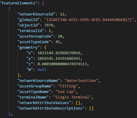
Things get more interesting when you look at a device that has two (or more) terminals. In the map this will appear as a single feature, but in the export, it is represented as multiple elements. The export treats each terminal and terminal path as a separate feature.


This may seem a little unusual at first glance, but its importance is understood once you start comparing the contents of this file with the connectivity portions of the JSON file which reference the individual terminal and edges to establish connectivity. To uniquely identify each point element in the JSON file we could use the network source id, object id, and terminal id of the feature (which would match the connectivity). However, you will notice that in our parser we have chosen to uniquely identify each feature using just the network source id and object id of each feature. This reduces redundancy and means that to look up attribute information you need only a network source id and object id.
feature_key = f"{element['networkSourceId']}${element['objectId']}"
The next difference you will note is in how line features are represented. This is because, in the utility network, each line feature is represented by one or more edge elements. When a line has midspan connectivity then the network uses multiple edge elements to represent each of the sections of the line. You can see this in the example below where the line feature in our geodatabase has two feature elements in the file, each representing a different segment of the line.


To uniquely identify the attributes of each feature, it is sufficient to consider the network source id and object id of the feature. However, to consolidate the geometries for the feature we must consider the from position and to position of each edge because each JSON element represents a subset of the overall line’s geometry. Using the example from above we can see that the first segment accounts for 59% of the shape’s length, with the second segment accounting for the remaining 41%.
Similar to how we handled point features, our parser has chosen to consolidate all the attributes for edge elements into a single feature using the network source id and object id. For the geometries however, we are storing the “from position” of the JSON element along with the coordinates of the line so we can consolidate the geometries from multiple features into a single geometry.
Puedes ver la diferencia entre cómo estamos almacenando geometrías para características de punto y línea en el fragmento a continuación.
para clave, valor en element.items():
    si clave == "geometry":
        geometry_element = valor
        si "x" en geometry_element:
            # Crear un punto
            geometries[feature_key] = arcpy.Point(geometry_element["x"],geometry_element["y"],geometry_element["z"],geometry_element["m"])
        elif "fromPosition" en element:
            # Añadir la geometría del segmento de línea, junto con la posición en porcentaje
            # Usamos esto para unir todos los segmentos de línea más tarde
            other_geometries = geometries.get(feature_key, [])
            other_geometries.append([element["fromPosition"], geometry_element])
            geometries[feature_key] = other_geometries
Aunque no discutimos la creación de geometrías en este artículo, puedes mirar el método CreateGeometries en la herramienta adjunta para un ejemplo de cómo llenar una clase de entidad con las geometrías usando esta exportación. Si tu exportación no necesita usar información de geometría, puedes simplificar tu analizador y reducir considerablemente el tamaño de tu archivo simplemente excluyendo las geometrías de tu salida y haciendo que tu analizador las ignore.
Conectividad
El elemento "connectivity" en el archivo JSON es un grafo no dirigido que es una colección de nodos y aristas. Cada elemento de conexión describe una arista que conecta dos nodos donde los atributos from/to del elemento JSON se refieren a un nodo y los atributos via del elemento JSON hacen referencia a la arista.

Conectividad entre elementos
El script incluido muestra cómo lograr esto usando el método ProcessConnectivity. Este método analiza los elementos de conectividad en sus componentes separados from/via/to usando dos enfoques diferentes.
- Los elementos from y to están identificados de manera única por su id de fuente de red, id de objeto y su id terminal.
- Los elementos via están entonces identificados de manera única por el id de fuente de red, id de objeto, posición "from" y posición "to".
para element en connectivity_element:
    from_key = f"{element['fromNetworkSourceId']}${element['fromObjectId']}${element['fromTerminalId']}"
    to_key = f"{element['toNetworkSourceId']}${element['toObjectId']}${element['toTerminalId']}"
    via_key = f"{element['viaNetworkSourceId']}${element['viaObjectId']}${element['viaPositionFrom']}${element['viaPositionTo']}"
Una vez que todos los elementos from/via/to han sido analizados, podemos usar esta información para crear una lista de adyacencia. En el caso de este analizador, tratamos cada elemento from/via/to como su propio objeto y almacenamos las conexiones entre cada uno de ellos. Esta estructura es adecuada para análisis usando un algoritmo de recorrido de red, o para análisis usando bibliotecas Python como networkx.
# Almacenar la conectividad
from_connections = connectivity.get(from_key, [])
from_connections.append(via_key)

via_connections = connectivity.get(via_key, [])
via_connections.append(to_key)

# Si la conexión via es una asociación de conectividad, necesitamos añadir aristas a ambos lados
# Ya que no permitimos especificar dirección digitalizada en una asociación
si element["viaNetworkSourceId"] == 1:
    to_connections = connectivity.get(to_key, [])
    to_connections.append(via_key)
    connectivity[to_key] = to_connections

    via_connections.append(from_key)

connectivity[from_key] = from_connections
connectivity[via_key] = via_connections
Es importante recordar que la conectividad en este archivo JSON no posee direccionalidad, flujo ni información sobre transitabilidad. Más claramente, la direccionalidad implícita por el nombre de from, via y to no representa flujo real dentro de la red utility network, sino que representa el orden de los vértices en una línea o el origen/destino de la asociación (ninguno indica flujo). El flujo real de la utility network se calcula usando fuentes o sumideros cuando se realiza el rastreo y actualmente no se incluye en el JSON. Puedes ver un ejemplo de esto en el gráfico abajo donde algunas aristas parecen estar "invertidas". En esta área, el flujo real del agua va desde una zona de alta presión a la derecha hacia una zona de baja presión a la izquierda; sin embargo, la dirección digitalizada de las líneas en el mapa y JSON muestra el extremo "from" viniendo desde la izquierda hacia la derecha.

El elemento connectivity incluye geometrías para características similar al elemento features, lo que significa que cada elemento espacial from/via/to incluirá su geometría y el elemento edge geometry puede corresponder a un subconjunto de la geometría total para la arista si la característica edge contiene múltiples elementos edge como se ve abajo.
Ahora que hemos cubierto cómo procesar features y connectivity, la última pieza restante del rompecabezas es el elemento "associations".
{
    "viaNetworkSourceId": 10,
    "viaGlobalId": "{29C0B239-9AC0-4E76-9E5A-A912D46CF267}",
    "viaObjectId": 22258,
    "viaPositionFrom": 0.59016310696272389,
    "viaPositionTo": 1,
    "viaGeometry": {
        "hasZ": true,
        "hasM": true,
        "paths": [
            [
                [
                    1032056.63583742827,
                    1857139.22013278306,
                    0.00010000000474974513,
                    null
                ],
                [
                    1032024.145088762,
                    1857269.34913761169,
                    0.00010000000474974513,
                    null
                ]
            ]
        ]
    },
    "fromNetworkSourceId": 12,
    "fromGlobalId": "{6F988B32-CA53-4DE2-AA77-A79544386D3F}",
    "fromObjectId": 7271,
    "fromTerminalId": 1,
    "fromGeometry": {
        "x": 1032056.63583742827,
        "y": 1857139.22013278306,
        "z": 0.00010000000474974513,
        "m": null
    },
    "toNetworkSourceId": 12,
    "toGlobalId": "{4F36DEA2-656D-468D-B1F9-30849B04FC20}",
    "toObjectId": 7723,
    "toTerminalId": 1,
    "toGeometry": {
        "x": 1032024.145088762,
        "y": 1857269.34913761169,
        "z": 0.00010000000474974513,
        "m": null
    }
},
Associations
The “associations” JSON element is very similar to the “connectivity” element JSON in structure with the exception that each element consists of only a “from” and “to” element. Additionally, the utility network models associations at the feature level, so when cross-referencing associations to the features element you only need to consider the network source id and the global id of the “from” and “to” feature.
{
    "associationType": "containment",
    "fromNetworkSourceId": 6,
    "fromGlobalId": "{E4693E2A-441D-404F-871F-4D4C5E6AE20A}",
    "fromTerminalId": 1,
    "toNetworkSourceId": 9,
    "toGlobalId": "{FC1540AA-5965-4BDD-B207-F6AD0B40B5BE}",
    "toTerminalId": 1,
    "fromNetworkSourceName": "StructureBoundary",
    "fromTerminalName": "Single Terminal",
    "toNetworkSourceName": "WaterDevice",
    "toTerminalName": "Single Terminal"
},
By parsing the JSON this way, you can filter out what appear as duplicate associations. Doing this before outputting your results will make it easier to interpret your results as well as reduce the size of any files you output.
{
    "associationType": "containment",
    "fromNetworkSourceId": 5,
    "fromGlobalId": "{8F686F75-3E07-4EFA-BAA4-EAE03F40D93F}",
    "fromTerminalId": -1,
    "toNetworkSourceId": 10,
    "toGlobalId": "{92D69B81-FF17-4C5A-85CB-0733AFE8F02A}",
    "toTerminalId": -1,
    "fromNetworkSourceName": "StructureLine",
    "fromTerminalName": "",
    "toNetworkSourceName": "WaterLine",
    "toTerminalName": ""
},
… association repeats multiple times …
{
    "associationType": "containment",
    "fromNetworkSourceId": 5,
    "fromGlobalId": "{8F686F75-3E07-4EFA-BAA4-EAE03F40D93F}",
    "fromTerminalId": -1,
    "toNetworkSourceId": 10,
    "toGlobalId": "{92D69B81-FF17-4C5A-85CB-0733AFE8F02A}",
    "toTerminalId": -1,
    "fromNetworkSourceName": "StructureLine",
    "fromTerminalName": "",
    "toNetworkSourceName": "WaterLine",
    "toTerminalName": ""
},
Note that because we are referencing associations by network source id and global id, while referencing other features by their network source id and object id we will need to do some translation when comparing the different datasets. In this example, the use of the object id was a deliberate choice to make it simpler to select and interact with the geodatabase, but for other applications it may be easier to not use object id for any comparisons and just use the global id.
Conclusion
Now that you have read this article you are equipped with a better understanding of interpreting and parsing the features, connectivity, and associations elements in JSON files produced by the utility network. To inspire you further, attached to this article is a sample Python tool that demonstrates how these techniques can be used to craft your own custom analysis. Happy parsing!