GIS Life Blog

cancel
Showing results for 
Show  only  | Search instead for 
Did you mean: 

Other Boards in This Place

Latest Activity

(450 Posts)
JoshuaBixby
MVP Esteemed Contributor

Don Knuth is often quoted as saying, "premature optimization is the root of all evil" when it comes to computer programming.  Attribution usually comes from "Structured Programming with go to Statements," a journal article he published in the mid-1970s.  Although the phrase makes for a great soundbite, I think his entire explanation makes the point better:

There is no doubt that the grail of efficiency leads to abuse.  Programmers waste enormous amounts of time thinking about, or worrying about, the speed of noncritical parts of their programs, and these attempts at efficiency actually have a strong negative impact when debugging and maintenance are considered.  We should forget about small efficiencies, say about 97% of the time: premature optimization is the root of all evil.

The trick to optimizing code is to learn when you are chasing the 97% tail versus getting to the 3% heart of it.  Experience helps greatly with answering that question but so can simple tests and empirical data.


When scripting with Python geometry libraries (ArcPy, ArcGIS API for Python, Shapely, GeoDjango, etc....), it is quite common to encounter Python lists containing geometry coordinates, and turning those coordinates into geometry objects involves calling geometry constructors.  For ArcPy geometry classes, like most Python classes, the default constructor is accessed by calling the class and passing arguments.  For Polygon—ArcPy classes | ArcGIS Desktop:

Syntax

Polygon  (inputs, {spatial_reference}, {has_z}, {has_m})
ParameterExplanationData Type
inputs

The coordinates used to create the object. The data type can be either Point or Array objects.

Object
spatial_reference  

The spatial reference of the new geometry.

(The default value is None)

SpatialReference
has_z  

The Z state: True for geometry if Z is enabled and False if it is not.

(The default value is False)

Boolean
has_m  

The M state: True for geometry if M is enabled and False if it is not.

(The default value is False)

Boolean

In addition to the ArcPy geometry class constructors, there are several other constructors for creating ArcPy geometries:


Given there are multiple ways to construct ArcPy geometries, it is reasonable for someone to wonder which constructor they should or shouldn't use.  The descriptions of arcpy.FromWKT(), arcpy.FromWKB(), and arcpy.AsShape() tell us those constructors work with specific geometry representations or encodings.  When it comes to which constructor someone should use, I think Don Knuth would argue the one that most closely matches your data's existing structure, i.e., don't overthink it.

I recently had reason to overthink ArcPy geometry constructors, or thought I had reason to, so I set about running some basic timing tests to gather more information before deciding whether to refactor some code involving arcpy.Polygon().  Using the simple, multipart polygon from /blogs/tilting/2017/06/10/a-case-of-missing-prefixes-esris-geometries?sr=search&searchId=1171f7ce-f9...‌,

I created four tests constructing the geometry from a Python list containing coordinates:


import arcpy
import timeit

poly_rings = [
    [[15,0], [25,0], [25,10], [15,10], [15,0]],
    [[18,13], [24,13], [24,18], [18,18], [18,13]
]]

def FromArcPyArray():
    aarr = arcpy.Array(
        arcpy.Array(arcpy.Point(*xy) for xy in ring) for ring in poly_rings
    )
    return arcpy.Polygon(aarr)

def FromEsriJSON():
    esri_json = {"type":"Polygon", "rings":poly_rings}
    return arcpy.AsShape(esri_json, True)

def FromGeoJSON():
    geojson = {"type":"Polygon", "coordinates":poly_rings}
    return arcpy.AsShape(geojson)

def FromWKT():
    wkt = "MULTIPOLYGON({})".format(
        ",".join("(({}))".format(
            ", ".join("{} {}".format(*xy) for xy in ring)
        ) for ring in poly_rings)
    )
    return arcpy.FromWKT(wkt)‍‍‍‍‍‍‍‍‍‍‍‍‍‍‍‍‍‍‍‍‍‍‍‍‍‍‍‍‍‍‍‍‍‍‍‍‍‍‍‍‍‍‍‍‍‍‍‍‍‍‍‍‍‍‍‍‍‍‍‍‍‍‍‍‍
‍‍‍‍‍‍‍‍‍‍‍‍‍‍‍‍‍‍‍‍‍‍‍‍‍‍‍‍‍‍‍‍‍‍‍‍‍‍‍‍‍‍‍‍‍‍‍‍‍‍‍‍‍‍‍‍‍‍‍‍‍‍‍‍‍‍‍‍‍‍‍‍‍‍‍‍‍‍‍‍‍‍‍‍‍‍‍‍‍


Using 26.6. timeit — Measure execution time of small code snippets — Python 2.7.15 documentation from Python 2.7.14 bundled with ArcGIS Desktop 10.6.1:


>>> for ctor in [FromArcPyArray, FromEsriJSON, FromGeoJSON, FromWKT]:
...     pg = ctor()
...     print("\n".join(
...         str(i) for i in [ctor.__name__, timeit.timeit(ctor, number=10000), ""]
...     ))
...
FromArcPyArray
20.2141071389

FromEsriJSON
4.77303549343

FromGeoJSON
20.2831866771

FromWKT
4.03049759916

>>> ‍‍‍‍‍‍‍‍‍‍‍‍‍‍‍‍‍‍‍‍‍‍‍‍‍‍‍‍‍‍‍‍‍‍‍‍‍‍‍‍‍‍‍‍‍‍‍‍‍‍‍‍‍‍‍‍‍‍‍‍‍‍‍‍‍‍‍‍‍‍‍‍‍‍‍‍


I must admit, the results aren't what I was expecting.  I expected some timing differences between the various constructors, but I didn't expect some to be 5x faster than others.  What I really didn't expect is the ArcPy Polygon constructor nearly being the slowest.

Since I have ArcGIS Desktop 10.6.1 and ArcGIS Pro 2.2.3 on the same machine, I just had to run the same tests using 27.5. timeit — Measure execution time of small code snippets — Python 3.6.7 documentation from Python 3.6.5 bundled with ArcGIS Pro 2.2.3:


>>> for ctor in [FromArcPyArray, FromEsriJSON, FromGeoJSON, FromWKT]:
...     pg = ctor()
...     print("\n".join(
...         str(i) for i in [ctor.__name__, timeit.timeit(ctor, number=10000), ""]
...     ))
...
FromArcPyArray
10.2499491093713

FromEsriJSON
0.9167164168891304

FromGeoJSON
9.85043158674398

FromWKT
0.5525892638736423

>>> ‍‍‍‍‍‍‍‍‍‍‍‍‍‍‍‍‍‍‍‍‍‍‍‍‍‍‍‍‍‍‍‍‍‍‍‍‍‍‍‍‍‍‍‍‍‍‍‍‍‍‍‍‍‍‍‍‍‍‍‍‍‍‍‍‍‍‍‍‍‍‍‍‍‍‍‍


What?!  This goes beyond unexpected, this is outright surprising.  It is good to see a nearly 50% decrease in the ArcPy Polygon constructor, but it is amazing to see 80% and 85% decreases in Esri JSON and WKT constructors.  The Esri JSON constructor went from 4x to 11x faster than the ArcPy Polygon constructor, and the WKT constructor is now 19x faster!

When basic timing tests come back with results this surprising, one has to wonder whether the relative timing differences will hold up when the tests use larger, real-world data.  To answer that question, I downloaded the USA States layer package included with Esri Data & Maps and available on ArcGIS.com.  I wanted a multipart polygon, and Michigan was the first state that came to mind.  It turns out, because of all the small islands in the Great Lakes, Michigan is a very multipart polygon:  450 parts and 166,107 points.


>>> for ctor in [FromArcPyArray, FromEsriJSON, FromGeoJSON, FromWKT]:
...     pg = ctor()
...     print("\n".join(
...         str(i) for i in [ctor.__name__, timeit.timeit(ctor, number=100), ""]
...     ))
...
FromArcPyArray
1267.5038210736802

FromEsriJSON
141.83130611867819

FromGeoJSON
464.2651427417986

FromWKT
86.92622569438026

>>> ‍‍‍‍‍‍‍‍‍‍‍‍‍‍‍‍‍‍‍‍‍‍‍‍‍‍‍‍‍‍‍‍‍‍‍‍‍‍‍‍‍‍‍‍‍‍‍‍‍‍‍‍‍‍‍‍‍‍‍‍‍‍‍‍‍‍‍‍‍‍‍‍‍‍‍‍


For the most part, the relative results stay consistent when using a larger and more complex multipart polygon.  The ArcPy Polygon constructor does scale slightly better than the Esri JSON and WKT constructors, going from 11x and 19x slower to 9x and 15x slower respectively, but those improvements aren't nearly enough to make up for the overall slowness of the constructor.

Overall, I don't really know what to think about the GeoJSON constructor.  With small and simple polygons, it is as slow or slower than the ArcPy Polygon constructor.  With larger polygons it scales better than all of the other constructors, in relative terms, but it is still quite slow overall.

Comparing the timings between the simple example polygon and the Michigan polygon, the constructors appear to scale roughly linearly with the number of points/vertices in the polygon.  For the Michigan polygon the number of iterations was lowered 2 orders of magnitude (10,000 to 100) while the run times increased by roughly 2 orders of magnitude, leading to run times that are 4 orders of magnitude longer.  The magnitude of increase in run times is matched by an equal magnitude of increase points/vertices (10 to 166,107).

The results of these tests surprised me, truly.  I am not going to wholesale abandon the ArcPy geometry default constructors, but I do think they are worth a solid look when optimizing code.

more
7 3 1,510
JoshuaBixby
MVP Esteemed Contributor

As I raise in /blogs/tilting/2016/09/27/performance-at-a-price-file-geodatabases-and-sql-support, Esri made trade offs when developing the file geodatabase as a replacement or upgrade to the personal geodatabase.  One of the biggest trade offs was and continues to be support for SQL.  In /blogs/tilting/2016/10/04/when-exists-doesnt-file-geodatabases-and-correlated-subqueries I provide one example where Esri partially implements an SQL operator.

While partially implementing a standard isn't unusual, partially implementing a distinct component or aspect of a standard is unusual.  In Esri's case with EXIST and SQL, it would have been better to not implement EXIST at all than partially implement it and allow for common SQL patterns with it to generate incorrect results.

Another part of SQL support lacking in the file geodatabase is expanded pattern matching for strings.  I have lamented the lack of such functionality in GeoNet responses from time to time, and I have even went so far as to log enhancement requests with Esri Support and submit an ArcGIS Idea (Expanded Pattern Matching in File Geodatabases (and documentation would be nice ), but it all seemed for naught, until a few months ago....

It turns out Esri has implemented SQL support for expanded pattern matching in file geodatabases, they just haven't told anyone about it. So how long has this support been around and what all is supported?  Both good questions.  It would be great to get answers directly from Esri, but let's not hold our breaths given that the file geodatabase has been around for almost 12 years and Esri has never said a peep yet about expanded pattern matching support.

With respect to the first question, i.e., how long has expanded pattern matching support been included, I experimented back to ArcGIS 9.3 (I could not find ArcGIS 9.2 installer files to go all the way back to the introduction of the file geodatabase).  As interesting as my experimentation was, there is too much to include here.  Suffice it to say, what I share below only works properly in ArcGIS Desktop 10.6 or greater and ArcGIS Pro 2.0 and greater.

Unlike basic pattern matching using LIKE, expanded pattern matching is implemented using a range of operators/predicates:

In terms of expanded pattern matching and the file geodatabase, Esri has chosen the SIMILAR predicate, which was originally codified in ISO/IEC 9075-1:1999.  Although PostgreSQL implements SIMILAR as well (see PostgreSQL: Documentation: 9.3: Pattern Matching), I have found several important cases where supported functionality in PostgreSQL does not work in the file geodatabase.  To date, the Firebird documentation on SIMILAR TO comes the closest of describing the behavior I have seen with the file geodatabase.

So, what does this all mean for querying feature classes and tables in a file geodatabase?  Instead of making up some data to demonstrate the functionality, let's use someone's data and their question from a GeoNet post:  ArcGIS Select Query help.

First step, build a scratch table containing the data to query:

>>> import arcpy
>>> 
>>> field = {'field_name':'Field1', 'field_type':'TEXT', 'field_length':24}
>>> values = [
...     'A1,F4,A10',
...     'A1,A17',
...     'F1,G6, A1',
...     'A10, A1',
...     'D1, A17',
...     'D2, D4',
...     'A1 ,D2',  # value not included in original post, added for demonstration 
...     'G6, A10'  # value not included in original post, added for demonstration
... ]
... 
>>> scratchGDB = arcpy.env.scratchGDB
>>> table = arcpy.CreateTable_management(scratchGDB, "tmpTable")
>>> arcpy.AddField_management(table, **field)
>>> with arcpy.da.InsertCursor(table, field['field_name']) as cur:
...     for value in values:
...         cur.insertRow([value])
...         
>>> 
>>> with arcpy.da.SearchCursor(table, "*") as cur:
...     for row in cur:
...         print(row)
...         
(1, u'A1,F4,A10')
(2, u'A1,A17')
(3, u'F1,G6, A1')
(4, u'A10, A1')
(5, u'D1, A17')
(6, u'D2, D4')
(7, u'A1 ,D2')
(8, u'G6, A10')
>>> 
>>> del row, cur, value
>>> field = field['field_name']
>>> 
>>> # create helper function to select and print records using cursor
>>> def select_and_print(table, where_clause):
...     with arcpy.da.SearchCursor(table, "*", where_clause) as cur:
...         for row in cur:
...             print(row)
...             
>>> ‍‍‍‍‍‍‍‍‍‍‍‍‍‍‍‍‍‍‍‍‍‍‍‍‍‍‍‍‍‍‍‍‍‍‍‍‍‍‍‍‍‍‍‍‍‍‍‍‍‍‍‍‍‍‍‍‍‍‍‍‍‍‍‍‍‍‍‍‍‍‍‍‍‍‍‍‍‍‍‍‍‍‍‍‍‍‍‍‍‍‍‍‍‍‍‍‍‍‍‍‍‍‍‍‍‍‍‍‍‍‍‍‍‍‍‍‍‍‍‍‍‍‍‍‍‍‍‍‍‍‍‍‍‍‍‍‍‍‍‍‍‍‍‍‍‍‍‍‍‍‍‍‍‍‍‍‍‍‍‍‍‍‍‍‍‍‍‍‍‍‍‍‍‍‍‍‍‍‍‍‍‍‍‍‍‍‍‍‍‍‍‍‍‍‍‍‍‍‍‍‍‍‍‍‍‍‍‍‍‍‍‍‍‍‍‍‍‍‍‍‍‍‍‍‍‍‍‍‍‍‍‍‍‍‍‍‍‍‍‍‍‍‍‍‍‍‍‍‍‍‍‍‍‍‍‍‍‍‍‍‍‍‍‍‍‍‍‍‍‍‍‍‍‍‍‍‍‍‍‍‍‍‍‍‍‍‍‍‍‍‍‍‍‍‍‍‍‍‍‍‍‍‍‍‍‍‍‍‍‍‍‍‍‍‍‍‍‍‍‍‍‍‍‍‍‍‍‍‍‍‍‍‍‍‍‍‍‍‍‍‍‍‍‍‍‍‍‍‍‍‍‍‍‍‍‍‍‍‍‍‍‍‍‍‍‍‍‍‍‍‍‍‍‍‍‍‍‍‍‍‍‍‍‍‍‍‍‍‍‍‍‍‍‍‍‍‍‍‍‍‍‍‍‍‍‍‍‍‍‍‍‍‍‍‍‍‍‍‍‍‍‍‍‍‍‍‍‍‍‍‍‍‍‍‍‍‍‍‍‍‍‍‍‍‍‍‍‍‍‍‍‍‍‍‍‍‍‍‍‍‍‍‍‍‍‍‍‍‍‍‍‍‍‍‍‍‍‍‍‍‍‍‍‍‍‍‍‍‍‍‍‍‍‍‍‍‍‍‍‍‍‍‍‍‍‍‍‍‍‍‍‍‍‍‍‍‍‍‍‍‍‍‍‍‍‍‍‍‍‍‍‍‍‍‍‍‍‍‍‍‍‍‍‍‍‍‍‍‍‍‍‍‍‍‍‍‍‍‍‍‍‍‍‍‍‍‍‍‍‍‍‍‍‍‍‍‍‍‍‍‍‍‍‍‍‍‍‍‍‍‍‍‍‍‍‍‍‍‍‍‍‍‍‍‍‍‍‍‍‍‍‍‍‍‍‍‍‍‍‍‍‍‍‍‍‍‍‍‍‍

Now the question:

I am trying to select records showing A1 value.  I have tried using query  Field1 LIKE '%A1%', it is also selecting A10. Is there any way I can select only value A1?

Let's try what the user originally tried and see the result:

>>> sql = "{} LIKE '%A1%'".format(field)
>>> print(sql)
Field1 LIKE '%A1%'
>>> select_and_print(table, sql)
(1, u'A1,F4,A10')
(2, u'A1,A17')
(3, u'F1,G6, A1')
(4, u'A10, A1')
(5, u'D1, A17')
(7, u'A1 ,D2')
(8, u'G6, A10')
>>> ‍‍‍‍‍‍‍‍‍‍‍‍‍‍‍‍‍‍‍‍‍‍‍‍‍‍‍‍‍‍‍‍‍‍‍‍‍‍‍‍‍‍‍‍‍‍‍‍‍‍‍‍‍‍‍‍‍‍‍‍‍‍‍‍‍‍‍‍‍‍‍‍‍‍‍‍‍‍‍‍‍‍‍‍‍‍‍‍‍‍‍‍‍‍‍‍‍‍‍‍‍‍‍‍‍‍‍‍‍‍‍‍‍‍‍‍‍‍‍‍‍‍‍‍‍‍‍‍‍‍‍‍

We can see the problem the user was facing, i.e., basic SQL pattern matching (LIKE) using a wildcard (%) in front and behind the query value (A1) results in false-positive selections (A10 and A17). 

So if %A1% selects A10 and A17 in addition to A1, what if we put a comma after the value and before the wildcard:

>>> sql = "{} LIKE '%A1,%'".format(field)
>>> print(sql)
Field1 LIKE '%A1,%'
>>> select_and_print(table, sql)
(1, u'A1,F4,A10')
(2, u'A1,A17')
>>> ‍‍‍‍‍‍‍‍‍‍‍‍‍‍‍‍‍‍‍‍‍‍‍‍‍‍‍‍‍‍‍‍‍‍‍‍‍‍‍‍‍‍‍‍‍‍‍‍‍‍‍‍‍‍‍‍‍‍‍‍‍‍‍‍‍‍‍‍‍‍‍‍‍‍‍‍‍‍‍‍‍‍‍‍‍‍‍‍‍‍‍‍‍‍‍‍‍‍

Adding the comma definitely dropped the false-positive selections from before, but now certain records we want are not being selected, e.g., OID/record 3 and 7.

As you can start to see, there isn't a single basic pattern that will work in this situation.  In order to use basic pattern matching with LIKE, several predicates will need to be chained together.

>>> sql = ("{0} LIKE 'A1,%' OR\n"
...        "{0} LIKE 'A1 %' OR\n"
...        "{0} LIKE '% A1 %' OR\n"
...        "{0} LIKE '% A1,%' OR\n"
...        "{0} LIKE '%,A1 %' OR\n"
...        "{0} LIKE '%,A1,%' OR\n"
...        "{0} LIKE '% A1' OR\n"
...        "{0} LIKE '%,A1'").format(field)
...        
>>> print(sql)
Field1 LIKE 'A1,%' OR
Field1 LIKE 'A1 %' OR
Field1 LIKE '% A1 %' OR
Field1 LIKE '% A1,%' OR
Field1 LIKE '%,A1 %' OR
Field1 LIKE '%,A1,%' OR
Field1 LIKE '% A1' OR
Field1 LIKE '%,A1'
>>> select_and_print(table, sql)
(1, u'A1,F4,A10')
(2, u'A1,A17')
(3, u'F1,G6, A1')
(4, u'A10, A1')
(7, u'A1 ,D2')
>>> ‍‍‍‍‍‍‍‍‍‍‍‍‍‍‍‍‍‍‍‍‍‍‍‍‍‍‍‍‍‍‍‍‍‍‍‍‍‍‍‍‍‍‍‍‍‍‍‍‍‍‍‍‍‍‍‍‍‍‍‍‍‍‍‍‍‍‍‍‍‍‍‍‍‍‍‍‍‍‍‍‍‍‍‍‍‍‍‍‍‍‍‍‍‍‍‍‍‍‍‍‍‍‍‍‍‍‍‍‍‍‍‍‍‍‍‍‍‍‍‍‍‍‍‍‍‍‍‍‍‍‍‍‍‍‍‍‍‍‍‍‍‍‍‍‍‍‍‍‍‍‍‍‍‍‍‍‍‍‍‍‍‍‍‍‍‍‍‍‍‍‍‍‍‍‍‍‍‍‍‍‍‍‍‍‍‍‍‍‍‍‍‍‍‍‍‍‍‍‍‍‍‍‍‍‍‍‍‍‍‍‍‍‍‍‍‍‍‍‍‍‍‍‍‍‍‍‍‍‍‍‍‍‍‍‍‍‍‍‍‍‍‍‍‍‍‍‍‍‍‍

The possibility of spaces either before or after the value being queried means more conditions need to be addressed, which means more LIKE predicates.  For this data set, a total of 8 LIKE statements are needed to select the records of interest.

Since basic pattern matching with LIKE is implemented the same across database platforms, the code above is quite portable, even if it is a bit unwieldy and inefficient from a query execution perspective.  One can imagine the number of predicate statements getting really large, really quickly if the requirements for the query are more involved than our example here.

As the complexity of the data, search conditions, or both grows; expanded/complex pattern matching can be easier to implement and sometimes more efficient to execute.  Using the SIMILAR TO documentation from Firebird that I reference above, the following SQL statement can be used to query the records:

>>> sql = "{} SIMILAR TO '(A1[ ,]%|%[ ,]A1[ ,]%|%[ ,]A1)'".format(field)
>>> print(sql)
Field1 SIMILAR TO '(A1[ ,]%|%[ ,]A1[ ,]%|%[ ,]A1)'
>>> select_and_print(table, sql)
(1, u'A1,F4,A10')
(2, u'A1,A17')
(3, u'F1,G6, A1')
(4, u'A10, A1')
(7, u'A1 ,D2')
>>> ‍‍‍‍‍‍‍‍‍‍‍‍‍‍‍‍‍‍‍‍‍‍‍‍‍‍‍‍‍‍‍‍‍‍‍‍‍‍‍‍‍‍‍‍‍‍‍‍‍‍‍‍‍‍‍‍‍‍‍‍‍‍‍‍‍‍‍‍‍‍‍‍‍‍‍‍‍‍‍‍‍‍‍‍‍‍‍‍‍‍

Since SIMILAR is based on regular expression searching and the Firebird documentation appears to be fairly accurate/consistent with Esri's implementation, I will forgo explaining the structure of the SIMILAR statement above.  My intent with demonstrating the use of SIMILAR with file geodatabase data isn't to explain how regular expressions work, although I strongly encourage anyone who works with text data to learn regular expressions.

My goal with this blog post is to point out that Esri does support the use of SIMILAR in the file geodatabase, and that Esri really needs to document that support.

P.S. 

I would be remiss if I didn't point out Vince Angelo‌'s comment in ArcGIS Select Query help.  Although one can use text-based pattern matching to query values from lists that are stored in a field/column, such an approach is sub-optimal when it comes to working with relational data stores.  A more robust approach to structuring the data and querying it would be what Vince suggests:

If you had a second table organized:

keycolattrval
1A1
1F4
1A10
2A1
2A17
3F1
3G6
3A1
4A10
4A1


then you could fashion a query:

SELECT *

FROM mytable

WHERE keycol in (

   SELECT keycol

   FROM secondtab

   WHERE attrval = 'A1')


- V

more
2 0 1,063
JoshuaBixby
MVP Esteemed Contributor

My previous blog post, /blogs/tilting/2017/06/10/a-case-of-missing-prefixes-esris-geometries?sr=search&searchId=c6def5e0-70..., was unplanned.  I started writing this blog post and the next one, and I realized the background information I wanted to include didn't quite fit in either, so I wrote the background information up separately.

Over the years, I have found the ArcPy Geometry constructors to be quirky, especially with edge or niche cases like empty geometries.  As as engaged user, who believes providing feedback to developers is important, I have submitted several bugs and enhancement requests over time relating to geometry constructors.  Right off the top, I can't say how many have been implemented, possibly just one, but it wasn't one high up my wish list.

A couple years back I submitted the Support Empty Geometries with ArcPy Geometry Class Constructors idea.  Seeing how few users work with empty geometries, I can't say I am surprised with the whopping 2 votes it has received so far.  As‌ David Wynne from Esri points out in the comments, empty geometries are actually supported with the ArcPy Geometry constructors, it is just the syntax is undocumented.  Given empty geometries are supported by the constructors, I think my original idea should be merged under Pythonic ArcPy Geometries‌ since what I am really after is a more intuitive and idiomatic way to create empty geometries using ArcPy Geometry constructors.  I would merge my two ideas if I could, but I can't myself, and I don't want to just delete the idea.

Using the ArcPy Polygon class as an example, let's take a look at a variety of ways one might try to construct an empty geometry using the ArcPy Geometry constructors:

>>> ctor_stmts = (
...     '',
...     'None',
...     'arcpy.Array()',
...     'arcpy.Array(None)',
...     'arcpy.Point()',
...     'arcpy.Array([])',
...     'arcpy.Array([None])',
...     'arcpy.Array(arcpy.Array())',
...     'arcpy.Array(arcpy.Array(None))',
...     'arcpy.Array(arcpy.Array([]))'
... )
... 
>>> for i, stmt in enumerate(ctor_stmts):
...     stmt = "arcpy.Polygon({})".format(stmt)
...     try:
...         print("{:0>2}. {:<46}: {}".format(i+1, stmt, eval(stmt).WKT))
...     except Exception as err:
...         print("{:0>2}. {:<46}: {}....".format(i+1, stmt, err.message[:35]))
...         
01. arcpy.Polygon()                               : Object: CreateObject cannot create ....
02. arcpy.Polygon(None)                           : Object: CreateObject cannot create ....
03. arcpy.Polygon(arcpy.Array())                  : Object: CreateObject cannot create ....
04. arcpy.Polygon(arcpy.Array(None))              : MULTIPOLYGON EMPTY
05. arcpy.Polygon(arcpy.Point())                  : MULTIPOLYGON EMPTY
06. arcpy.Polygon(arcpy.Array([]))                : Object: CreateObject cannot create ....
07. arcpy.Polygon(arcpy.Array([None]))            : MULTIPOLYGON EMPTY
08. arcpy.Polygon(arcpy.Array(arcpy.Array()))     : MULTIPOLYGON EMPTY
09. arcpy.Polygon(arcpy.Array(arcpy.Array(None))) : MULTIPOLYGON EMPTY
10. arcpy.Polygon(arcpy.Array(arcpy.Array([])))   : MULTIPOLYGON EMPTY
>>> ‍‍‍‍‍‍‍‍‍‍‍‍‍‍‍‍‍‍‍‍‍‍‍‍‍‍‍‍‍‍‍‍‍‍‍‍‍‍‍‍‍‍‍‍‍‍‍‍‍‍‍‍‍‍‍‍‍‍‍‍‍‍‍‍‍‍‍‍‍‍‍‍‍‍‍‍‍‍‍‍‍‍‍‍‍‍‍‍‍‍‍‍‍‍‍‍‍‍‍‍‍‍‍‍‍‍‍‍‍‍‍‍‍‍‍‍‍‍‍‍‍‍‍‍‍‍‍‍‍‍‍‍‍‍‍‍‍‍‍‍‍‍‍‍‍‍‍‍‍‍‍‍‍‍‍‍‍‍‍‍‍‍‍‍‍‍‍‍‍‍‍‍‍‍‍‍‍‍‍‍‍‍‍‍‍‍‍‍‍‍‍‍‍‍‍‍‍‍‍‍‍‍‍‍‍‍‍‍‍‍‍‍‍‍‍‍‍‍‍‍‍‍‍‍‍‍‍‍‍‍‍‍‍‍‍‍‍‍‍‍‍‍‍‍‍‍‍‍‍‍‍‍‍‍‍‍‍‍‍‍‍‍‍‍‍‍‍‍‍‍‍‍‍‍‍‍‍‍‍‍‍‍‍‍‍‍‍‍‍‍‍‍‍‍‍‍‍‍‍‍‍‍‍‍‍‍‍‍‍‍‍‍‍‍‍‍‍‍‍‍‍‍‍‍‍‍‍‍‍‍‍‍‍‍‍‍‍‍‍‍‍‍‍‍‍‍‍‍‍‍‍‍‍‍‍‍‍‍‍‍‍‍‍‍‍‍‍‍‍‍‍‍‍‍‍‍‍‍‍‍‍‍‍‍‍‍‍‍‍‍‍‍‍‍‍‍‍‍‍‍‍‍‍

Before sharing any thoughts or comments, I think it is important to refresh ourselves on exactly what the ArcPy Polygon documentation states:

Syntax

 Polygon  (inputs, {spatial_reference}, {has_z}, {has_m})
ParameterExplanationData Type
inputs

The coordinates used to create the object. The data type can be either Point

or Array objects.

Object

A few observations before comments:

  • Examples 01 & 02:
    • The documentation states the inputs need to be Point or Array objects, which neither of these examples provide.
  • Examples 03 & 06:
    • These two examples are the same, e.g., repr(arcpy.Array()) == repr(arcpy.Array([]))Since Esri doesn't implement equivalence with ArcPy Arrays, I used the objects' __repr__ to show equality in this case.
    • Calling arcpy.Array() creates an empty ArcPy Array:  <Array []>.  Empty ArcPy Arrays are valid objects, and the documentation states ArcPy Array objects can be passed to the ArcPy Polygon constructor.
  • Examples 04 & 07:
  • Example 05:
    • The documentation states a Point object can be used as an input.
    • Calling arcpy.Point() doesn't create an empty point, like calling arcpy.Array(), instead it creates a 0, 0 point: <Point (0.0, 0.0, #, #)>.  Although not demonstrated above, further testing shows any point works, e.g., arcpy.Polygon(arcpy.Point(10000.5, -4500.3)) also creates an empty multi-polygon.
  • Examples 08 & 10:
    • Similar to Examples 03 & 06 and Examples 04 & 07, these two examples are the same.
    • Calling arcpy.Array(arcpy.Array()) creates an empty ArcPy Array nested within an ArcPy Array.  The ArcPy Array documentation does state an ArcPy Array is a valid input to the ArcPy Array constructor.

There are several oddities with the results from the polygon constructor test above.  I think Examples 03 & 06 are most likely to trip users up.  The documentation clearly states ArcPy Array objects are valid inputs, and empty ArcPy Arrays are valid objects, so why does passing an empty ArcPy Array to the ArcPy Polygon constructor generate an error?  Although Examples 04 & 07 work, it does seem odd that an ArcPy Array containing a Python None is somehow substantively different than an empty ArcPy Array when building an empty geometry.

Example 05 is a surprise and makes the least sense to me.  The documentation clearly states a Point object is a valid input to the ArcPy Polygon constructor, but what does a polygon with a single point look like?  An empty multi-polygon, according to Esri.  What takes the strangeness up another level for me is that there is no empty ArcPy Point, and that any ArcPy Point that is passed to the ArcPy Polygon constructor creates an empty geometry.

Using dis — Disassembler for Python bytecode to look at the bytecode for each of the constructor statements above, it appeared Example 05 would be the highest performing constructor statement.  Running timeit — Measure execution time of small code snippets on the constructor statements showed Example 05 was the quickest at generating empty geometries, not by much, but still the quickest.  This only adds to the mystery of the single-point polygon.

Examples 08 & 10 will be touched on in a subsequent blog post, so I won't dive into my thoughts on them here.

So how do the results from this test fit into the idea/request/plea for more Pythonic ArcPy Geometries‌?  For me, the answer is that Example 01 should be the primary way to create ArcPy empty geometries, i.e., passing no arguments to an ArcPy Geometry constructor should generate the equivalent empty geometry type.  For objects that support the concept of emptiness, it is fairly common in Python to have passing no arguments to the constructor create an empty object.  Let's look at some examples:

>>> # Common built-in data structures
>>> list()
[]
>>> set()
set([])
>>> dict()
{}
>>> str()
''
>>> 
>>> # Some SciPy data structures now bundled with ArcGIS
>>> import pandas
>>> pandas.DataFrame()
Empty DataFrame
Columns: []
Index: []
>>> import matplotlib.pylab
>>> matplotlib.pylab.plot()
[]
>>> ‍‍‍‍‍‍‍‍‍‍‍‍‍‍‍‍‍‍‍‍‍‍‍‍‍‍‍‍‍‍‍‍‍‍‍‍‍‍‍‍

What is more Pythonic for creating an empty geometry, arcpy.Polygon(arcpy.Array(None)) or arcpy.Polygon() ?

UPDATE 06/2018:

For the sake of completeness, I want to include the results of running the constructor tests on the other ArcPy Geometry classes:

>>> geometry_classes = ["point", "multipoint", "polyline"]
>>> ctor_stmts = (
    '',
    'None',
    'arcpy.Array()',
    'arcpy.Array(None)',
    'arcpy.Point()',
    'arcpy.Array([])',
    'arcpy.Array([None])',
    'arcpy.Array(arcpy.Array())',
    'arcpy.Array(arcpy.Array(None))',
    'arcpy.Array(arcpy.Array([]))'
)
>>> for geometry in geometry_classes:
...     for i, stmt in enumerate(ctor_stmts):
...         stmt = "arcpy.Geometry('{}',{})".format(geometry, stmt)
...         try:
...             print("{:0>2}. {:<60}: {}".format(i+1, stmt, eval(stmt).WKT))
...         except Exception as err:
...             print("{:0>2}. {:<60}: {}....".format(i+1, stmt, err.message[:20]))
...     print("")
...     
01. arcpy.Geometry('point',)                                    : Object: CreateObject....
02. arcpy.Geometry('point',None)                                : Object: CreateObject....
03. arcpy.Geometry('point',arcpy.Array())                       : Object: CreateObject....
04. arcpy.Geometry('point',arcpy.Array(None))                   : Object: CreateObject....
05. arcpy.Geometry('point',arcpy.Point())                       : POINT (0 0)
06. arcpy.Geometry('point',arcpy.Array([]))                     : Object: CreateObject....
07. arcpy.Geometry('point',arcpy.Array([None]))                 : Object: CreateObject....
08. arcpy.Geometry('point',arcpy.Array(arcpy.Array()))          : Object: CreateObject....
09. arcpy.Geometry('point',arcpy.Array(arcpy.Array(None)))      : Object: CreateObject....
10. arcpy.Geometry('point',arcpy.Array(arcpy.Array([])))        : Object: CreateObject....

01. arcpy.Geometry('multipoint',)                               : Object: CreateObject....
02. arcpy.Geometry('multipoint',None)                           : Object: CreateObject....
03. arcpy.Geometry('multipoint',arcpy.Array())                  : Object: CreateObject....
04. arcpy.Geometry('multipoint',arcpy.Array(None))              : MULTIPOINT EMPTY
05. arcpy.Geometry('multipoint',arcpy.Point())                  : MULTIPOINT ((0 0))
06. arcpy.Geometry('multipoint',arcpy.Array([]))                : Object: CreateObject....
07. arcpy.Geometry('multipoint',arcpy.Array([None]))            : MULTIPOINT EMPTY
08. arcpy.Geometry('multipoint',arcpy.Array(arcpy.Array()))     : MULTIPOINT EMPTY
09. arcpy.Geometry('multipoint',arcpy.Array(arcpy.Array(None))) : MULTIPOINT EMPTY
10. arcpy.Geometry('multipoint',arcpy.Array(arcpy.Array([])))   : MULTIPOINT EMPTY

01. arcpy.Geometry('polyline',)                                 : Object: CreateObject....
02. arcpy.Geometry('polyline',None)                             : Object: CreateObject....
03. arcpy.Geometry('polyline',arcpy.Array())                    : Object: CreateObject....
04. arcpy.Geometry('polyline',arcpy.Array(None))                : MULTILINESTRING EMPTY
05. arcpy.Geometry('polyline',arcpy.Point())                    : MULTILINESTRING EMPTY
06. arcpy.Geometry('polyline',arcpy.Array([]))                  : Object: CreateObject....
07. arcpy.Geometry('polyline',arcpy.Array([None]))              : MULTILINESTRING EMPTY
08. arcpy.Geometry('polyline',arcpy.Array(arcpy.Array()))       : MULTILINESTRING EMPTY
09. arcpy.Geometry('polyline',arcpy.Array(arcpy.Array(None)))   : MULTILINESTRING EMPTY
10. arcpy.Geometry('polyline',arcpy.Array(arcpy.Array([])))     : MULTILINESTRING EMPTY

>>> ‍‍‍‍‍‍‍‍‍‍‍‍‍‍‍‍‍‍‍‍‍‍‍‍‍‍‍‍‍‍‍‍‍‍‍‍‍‍‍‍‍‍‍‍‍‍‍‍‍‍‍‍‍‍‍‍

arcpy.Polyline() behaves the same as arcpy.Polygon() while arcpy.Multipoint() has one difference with passing arcpy.Point()

more
3 5 1,371
JoshuaBixby
MVP Esteemed Contributor

In /blogs/tilting/2014/07/25/semantic-overloading, I touch on one of the main motivations for writing the Tilting at Globes blog:

I believe semantics are important in all aspects of life.  Whether in law, medicine, science, business, information technology, or any other field; having a common language doesn't do much good if there isn't a common understanding of the words that make up the language.  Since languages evolve, maintaining a common understanding of words over time is a continual challenge.

Ideally, a common understanding would mean a word or term has a single meaning, and that singular meaning is known and understood by all that use the word or term.  Unfortunately, reality isn't always ideal, and sometimes the context of the word or term plays a large part in its meaning.  For example, how the term "large-scale" is applied to maps can seem counter intuitive to how it is applied to actions, events, and typical objects.  When one understands that map scale applies to the representation of data in the map, i.e., the ratio of distance in the map to distance on the ground, it helps explain why "large-scale" maps cover small geographic areas instead of large geographic areas.  Sure, a large-scale map could cover a large geographic area if printed on an enormous medium, but I am assuming typical print sizes.

Moving from maps to geometries, I bring up a case of spatial operators in /blogs/tilting/2015/05/14/whats-within-when-esri-clementini .  In the blog post, I point out how the answer to whether one geometry is "within" another geometry can depend on whom you ask, or more accurately, whose definition of "within" is used to answer the question.  Often times, the qualifiers are either incomplete or left off of the answers entirely, and we end up relying on context to fill in the gaps.

In addition to how geometries relate to each other, there are even different contexts for understanding the structure of geometries or geometry types.  Esri's current-generation ArcGIS Geometry Object Model has been around since the release of ArcMap 8.0.  Although the model has evolved some over time, it is not significantly different than when it was released in 1999.  I am not clear on the history of Esri's ST_Geometry storage type, but I know it has been around since at least the ArcGIS 9.x days.  Even operating within a context of Esri geometry types, dropping qualifiers can lead to ambiguity at times.  It can be argued that Esri's REST API represents a 3rd Esri geometry model, but adding that geometry model into this blog post doesn't change the observations and conclusions.

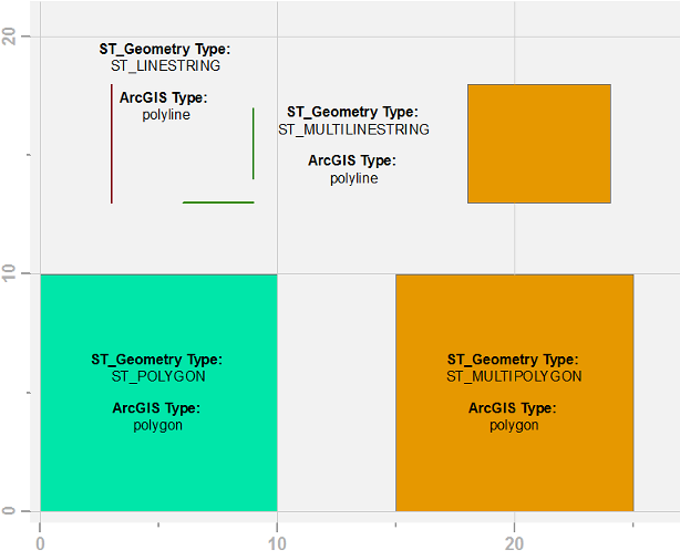
Instead of diving into object model diagrams and reference documentation, let's look at an example of how ArcGIS and ST_Geometry types differ in terms of structure.   Below is an image of, and the code to create, four geometries in a SQLite database using Esri's ST_Geometry type.  Each geometry is attributed with both its ST_Geometry and ArcGIS geometry type.

ArcMap layout with ST_Geometry sample geometries

import arcpy
import os
import sqlite3
from itertools import chain

# Define geometry samples
PCSCode = 3857
geoms = [
    ("poly", "polygon", "POLYGON((0 0, 10 0, 10 10, 0 10, 0 0))"),
    ("multipoly", "multipolygon", ("MULTIPOLYGON(((15 0, 25 0, 25 10, 15 10, 15 0)),"
                                           "((18 13, 18 18, 24 18, 24 13, 18 13)))")),
    ("line", "linestring", "LINESTRING(3 13, 3 18)"),
    ("multiline", "multilinestring", "MULTILINESTRING((6 13, 9 13),(9 14, 9 17))")
]

# Define SQLite database initialization parameters
sqlitedb = r"D:\tmp\test.sqlite" # path to SQLite DB
st_geometry_dll = r"DatabaseSupport\SQLite\Windows32\stgeometry_sqlite.dll"
st_geometry_dll = os.path.join(arcpy.GetInstallInfo()["InstallDir"],
                               st_geometry_dll)
sql_stmts = [[
        "SELECT load_extension('%s','SDE_SQL_funcs_init');" % st_geometry_dll
    ],[
        ("CREATE TABLE %s "
           "(id integer primary key autoincrement not null, "
             "stgeom_type text, arcgis_type text);" % table)
        for table, geom_type, WKT in geoms
    ],[
        ("SELECT AddGeometryColumn "
           "(null, '%s', 'geom', %s, '%s', 2, 'null');" % (table, PCSCode, geom_type))
        for table, geom_type, WKT in geoms
    ],[
        ("INSERT INTO %s "
           "(geom) VALUES (st_geometry('%s', %s));" % (table, WKT, PCSCode))
        for table, geom_type, WKT in geoms
    ],[
        ("UPDATE %s "
           "SET stgeom_type = st_geometrytype(geom);" % table)
        for table, geom_type, WKT in geoms
    ]
]

# Create SQLite database and setup tables
arcpy.CreateSQLiteDatabase_management(sqlitedb, "ST_GEOMETRY")
conn = sqlite3.Connection(sqlitedb)
conn.enable_load_extension(True)
cur = conn.cursor()
for sql in chain(*sql_stmts):
    cur.execute(sql)
conn.commit()
del cur, conn

# Populate ArcGIS geometry type
for table, geom_type, WKT in geoms:
    with arcpy.da.UpdateCursor(
        os.path.join(sqlitedb, table),
        ["shape@", "arcgis_type"]
    ) as cur:
        for shape, _ in cur:
            cur.updateRow([shape, shape.type])
del cur‍‍‍‍‍‍‍‍‍‍‍‍‍‍‍‍‍‍‍‍‍‍‍‍‍‍‍‍‍‍‍‍‍‍‍‍‍‍‍‍‍‍‍‍‍‍‍‍‍‍‍‍‍‍‍‍‍‍‍‍‍‍‍‍‍‍‍‍‍‍‍‍‍‍‍‍‍‍‍‍‍‍‍‍‍‍‍‍‍‍‍‍‍‍‍‍‍‍‍‍‍‍‍‍‍‍‍‍‍‍‍‍‍‍‍‍‍‍‍‍‍‍‍‍‍‍‍‍‍‍‍‍‍‍‍‍‍‍‍‍‍‍‍‍‍‍‍‍‍‍‍‍‍‍‍‍‍‍‍‍‍‍‍‍‍‍‍‍‍‍‍‍‍‍‍‍‍‍‍‍‍‍‍‍‍‍‍‍‍‍‍‍‍‍‍‍‍‍‍‍‍‍‍‍‍‍‍‍‍‍‍‍‍‍‍‍‍‍‍‍‍‍‍‍‍‍‍‍‍‍‍‍‍‍‍‍‍‍‍‍‍‍‍‍‍‍‍‍‍‍‍‍‍‍‍‍‍‍‍‍‍‍‍‍‍‍‍‍‍‍‍‍‍‍‍‍‍‍‍‍‍‍‍‍‍‍‍‍‍‍‍‍‍‍‍‍‍‍‍‍‍‍‍‍‍‍‍‍‍‍‍‍‍‍‍‍‍‍‍‍‍‍‍‍‍‍‍‍‍‍‍‍‍‍‍‍‍‍‍‍‍‍‍‍‍‍‍‍‍‍‍‍‍‍‍‍‍‍‍‍‍‍‍‍‍‍‍‍‍‍‍‍‍‍‍‍‍‍‍‍‍‍‍‍‍‍‍‍‍‍‍‍‍‍‍‍‍‍‍‍‍‍‍‍‍‍‍‍‍‍‍‍‍‍‍‍‍‍‍‍‍‍‍‍‍‍‍‍‍‍‍‍‍‍‍‍‍‍‍‍‍‍‍‍‍‍‍‍‍‍‍‍‍‍‍‍‍‍‍‍‍‍‍‍‍‍‍‍‍‍‍‍‍‍‍‍‍‍‍‍‍‍‍‍‍‍‍‍‍‍‍‍‍‍‍‍‍‍‍‍‍‍‍‍‍‍‍‍‍‍‍‍‍‍‍‍‍‍‍‍‍‍‍‍‍‍‍‍‍‍‍‍‍‍‍‍‍‍‍‍‍‍‍‍‍‍‍‍‍

A few observations:

  • ArcGIS has a single polyline geometry type, ST_Geometry has ST_LINESTRING and ST_MULTILINESTRING types.
  • ArcGIS has a single polygon geometry type, ST_Geometry has ST_POLYGON and ST_MULTIPOLYGON types.
  • Whereas ArcGIS has point and multipoint there is no multi- prefix when working with polyline and polygon.

If the ST_Geometry types look familiar to those who work with open standards, it isn't coincidence.  The documentation on How is ST_Geometry implemented?—Help | ArcGIS Desktop states in several places that ST_Geometry "is a high-performance storage type that includes ISO- and OGC-compliant SQL access to spatial data."  There are several ISO- and OGC- standards when it comes to geometries, and the "SQL access to spatial data" part of the statement is actually quite important as a qualifier.

ISO- and OGC-compliance is fairly broad across various geometry models or storage types, e.g., Microsoft's STGeometry, Oracle's SDO_GEOM,  PostGIS/PostgreSQL ST_Geometry, and others.  The OGC/OpenGIS geometry object model is described in OpenGIS® Implementation Standard for Geographic information - Simple feature access - Part 1: Common....  Instead of embedding a geometry class hierarchy diagram or listing all of the geometry types, I will share there are LineString and MultiLineString types as well as a Polygon and MultiPolygon types.

All of this leads to a point, and yes I do have a point, that ArcGIS polyline and polygon types are basically multi-types, just with the multi- prefix missing.  Worse yet, most of the ArcGIS documentation abstracts the user even further from the structure of the ArcGIS Geometry Object Model.  Instead of polylines having paths and polygons having rings, which they do, everything just has "parts."  I touch on this problem of "parts" in /blogs/tilting/2016/02/20/the-single-multipart-polygons-with-interior-boundaries:

The problem with the ArcPy Geometry classes, at least one of them, is that Esri replaced multiple, specific geometry components with a single generic one, the "part."  By abstracting geometries and rings with parts, not only did they deviate from geospatial standards and norms, they created the sideshow-worthy multi-part single-part polygon.

Whether it is missing prefixes or the ubiquitous part, understanding the nuances of the implementation and documentation of the ArcGIS Geometry Object Model can help one understand how ArcGIS software, including ArcPy, interacts with other geometry types.

more
3 0 1,196
JoshuaBixby
MVP Esteemed Contributor

In /blogs/tilting/2016/09/27/performance-at-a-price-file-geodatabases-and-sql-support?sr=search&searchI..., I bring attention to the SQL support trade-off Esri made while developing the file geodatabase (FGDB) as a replacement for the personal geodatabase (PGDB).  In that post, several links are provided for those who are interested in learning more about SQL support in file geodatabases.  Although there is plenty of overlap in content between the various sources/links, there are also important statements that only exist in one place or another, and knowing that can be important when troubleshooting errors or trying to understand spurious results from data stored in file geodatabases.

One area where users can get themselves into trouble with file geodatabases and SQL is the EXISTS condition or operator.  Looking at the SQL Reference (FileGDB_SQL.htm) in the File Geodatabase API ( @Esri Downloads ) or the SQL reference for query expressions used in ArcGIS:

[NOT] EXISTS

Returns TRUE if the subquery returns at least one record; otherwise, it returns FALSE. For example, this expression returns TRUE if the OBJECTID field contains a value of 50:

EXISTS (SELECT * FROM parcels WHERE "OBJECTID" = 50)
EXISTS is supported in file, personal, and ArcSDE geodatabases only.

Seeing that SQL EXISTS is supported in the file geodatabase, how does someone get himself into trouble using it?  Unfortunately, it is easier than you might expect, and the answer is correlated subqueries.

Correlated subqueries are fairly common when working with EXISTS, so common in fact that Microsoft's EXISTS (Transact-SQL) documentation and Oracle's EXISTS Condition documentation both use a correlated subquery in at least one code example.  At its simplest, a correlated subquery is a subquery that relates back to one or more tables in the outer query.  The theory and empiricism of correlated subqueries goes well beyond this blog post, but I will mention that correlated subqueries do have some JOIN-like properties, or at least appearances.

The following example is adapted from Select Max value arcpy‌, the same GeoNet question that got me researching this issue many months back.  Let's start with 2 basic tables (TableA and TableB), each having a text and integer field, and one table containing a subset of records from the other table.

A screenshot showing 2 basic tables with a handful of records

>>> fgdb = # path to file geodatabase
>>> pgdb = # path to personal geodatabase
>>> egdb = # path to enterprise geodatabase, SQL Server used in example
>>> gpkg = # path to GeoPackage
>>> gdbs = (fgdb, pgdb, egdb, gpkg)
>>> 
>>> values = (("A", 1), ("A", 2), ("B", 1), ("B", 2),
...           ("C", 2), ("C", 3), ("D", None), ("E", 1))
... 
>>> table_names = ("TableA", "TableB")
>>> 
>>> for gdb in gdbs:
...     for i in xrange(2,0,-1):
...         table = arcpy.CreateTable_management(gdb, table_names[i-1])
...         arcpy.AddField_management(table, "id", "TEXT")
...         arcpy.AddField_management(table, "version", "LONG")   
...         with arcpy.da.InsertCursor(table, ("id", "version")) as cur:
...             for value in values[::i]:
...                 cur.insertRow(value)
...     
...     qry = ("EXISTS (SELECT 1"
...                    "  FROM TableB"
...                    " WHERE TableB.id = TableA.id"
...                    "  AND TableB.version = TableA.version)")
...     
...     table_view = arcpy.MakeTableView_management(table, "table_view", qry)
...     print arcpy.GetCount_management(table_view)
...     arcpy.Delete_management(table_view)
0
3
3
3
>>> ‍‍‍‍‍‍‍‍‍‍‍‍‍‍‍‍‍‍‍‍‍‍‍‍‍‍‍‍‍‍‍‍‍‍‍‍‍‍‍‍‍‍‍‍‍‍‍‍‍‍‍‍‍‍‍‍‍‍‍‍‍‍‍‍‍‍‍‍‍‍‍‍‍‍‍‍‍‍‍‍‍‍‍‍‍‍‍‍‍‍‍‍‍‍‍‍‍‍‍‍‍‍‍‍‍‍‍‍‍‍‍‍‍‍‍‍‍‍‍‍‍‍‍‍‍‍‍‍‍‍‍‍‍‍‍‍‍‍‍‍‍‍‍‍‍‍‍‍‍‍‍‍‍‍‍‍‍‍‍‍‍‍‍‍‍‍‍‍‍‍‍‍‍‍‍‍‍‍‍‍‍‍‍‍‍‍‍‍‍‍‍‍‍‍‍‍‍‍‍‍‍‍‍‍‍‍‍‍‍‍‍‍‍‍‍‍‍‍‍‍‍‍‍‍‍‍‍‍‍‍‍‍‍‍‍‍‍‍‍‍‍‍‍‍‍‍‍‍‍‍‍‍‍‍‍‍‍‍‍‍‍‍‍‍‍‍‍‍‍‍‍‍‍‍‍‍‍‍‍‍‍‍‍‍‍‍‍‍‍‍‍‍‍‍‍‍‍‍‍‍‍‍‍‍‍‍‍‍‍‍‍‍‍‍‍‍‍‍‍‍‍‍‍‍‍‍‍‍‍‍‍‍‍‍‍‍‍‍‍‍‍‍‍‍‍‍‍‍‍‍‍‍‍‍‍‍‍‍‍‍‍‍‍‍‍‍‍‍‍‍‍‍‍‍‍‍‍‍‍‍‍‍‍‍‍‍‍‍‍‍‍‍‍‍‍‍‍‍‍‍‍‍‍‍‍‍‍‍‍‍‍‍‍‍‍‍‍‍‍‍‍‍‍‍‍‍‍‍‍‍‍‍‍‍‍‍‍‍‍‍‍‍

The sample code above creates the two basic tables in a file geodatabase, personal geodatabase, enterprise geodatabase (I used SQL Server), and a GeoPackage.  The code then creates a table view for each of the geodatabases by using EXISTS with a simple correlated subquery to select the records from TableA that have a matching id and version in TableB.  The correct table view is shown in the screenshot above.  One can see from the results of the code that no records are returned from the file geodatabase.

So why doesn't the file geodatabase return any records?  Are subqueries not supported?  Seeing that the documentation for EXISTS mentions subqueries, it seems they have to be supported, at least to some degree.  Let's take a closer look at the Subqueries section of SQL reference for query expressions used in ArcGIS:

Subqueries

Note:

Coverages, shapefiles, and other nongeodatabase file-based data sources do not support subqueries. Subqueries that are performed on versioned ArcSDE feature classes and tables will not return features that are stored in the delta tables. File geodatabases provide the limited support for subqueries explained in this section, while personal and ArcSDE geodatabases provide full support. For information on the full set of subquery capabilities of personal and ArcSDE geodatabases, refer to your DBMS documentation.

A subquery is a query nested within another query. It can be used to apply predicate or aggregate functions or to compare data with values stored in another table....

Subquery support in file geodatabases is limited to the following:

  • IN predicate. For example:
"COUNTRY_NAME" NOT IN (SELECT "COUNTRY_NAME" FROM indep_countries)
  • Scalar subqueries with comparison operators. A scalar subquery returns a single value. For example:
"GDP2006" > (SELECT MAX("GDP2005") FROM countries)

For file geodatabases, the set functions AVG, COUNT, MIN, MAX, and SUM can only be used within scalar subqueries.

  • EXISTS predicate. For example:
EXISTS (SELECT * FROM indep_countries WHERE "COUNTRY_NAME" = 'Mexico')

The documentation states "limited support" for subqueries, but it also states the EXISTS predicate is supported.  If subqueries aren't the problem, maybe correlated subqueries are the problem.  After all, none of the EXISTS examples in all of the documentation uses a correlated subquery.  Unfortunately, guessing is what we are left with because correlated subqueries are not mentioned explicitly in any of the file geodatabase documentation I can find.

From this simple example, it is clear the file geodatabase gives incorrect results when using EXISTS with correlated subqueries.  Are the incorrect results a bug or limitation of SQL support in the file geodatabase?  Even if one tries to argue the latter, there is still the problem of the user getting incorrect results instead of an error message, which should be what the user gets if correlated subqueries are not supported.

more
3 9 2,973
JoshuaBixby
MVP Esteemed Contributor

Between starting a new position and enjoying summer, it has been a while since I last blogged.  Although I do plan on finishing the Iterable Cursor series, I ran square into a limitation, and subsequent bug, of the file geodatabase that I thought worth sharing.  First, the limitation....

When the file geodatabase (FGDB) was introduced back in 2006, it was touted as an enhanced, high-performance alternative to the personal geodatabase (PGDB).  It is true that large data sets and large collections of data sets pose challenges for the personal geodatabase.  For one, Microsoft Access data files (*.mdb;*.accdb) are limited to 2 GB in size, which wasn't a whole lot in 2006 but is practically nothing today.  In addition to the file size limit, personal geodatabase performance starts to degrade around 500 MB of total data (see Types of geodatabases).  Another likely factor, but one Esri doesn't address, is the deprecation of the Jet database engine in the mid-2000s.

Taking a stroll down memory lane, or Esri Blogs as it may be, one finds Five reasons why you should be using the File Geodatabase:

Size

The database size is only limited by the available disk space. By default, individual tables and feature classes can be up to 1 TB. With the use of configuration keywords this can be expanded to 256 TB.

Versatility

Works on many different operating systems including Windows and UNIX (Solaris and Linux)

Speed

Provides excellent performance and scalability. For example, to support individual datasets containing well over 300 million features and datasets that can scale beyond 500 GB per file with very fast performance....

Edit Model

The File Geodatabase uses an edit model similar to shapefiles, supporting one editor and multiple readers.  Each standalone feature class, table and feature dataset can be edited by different editors simultaneously but can only have one editor performing edits on them at any given time....

Compression

File Geodatabases also allow users to compress feature classes and tables to a read-only format to reduce storage requirements even further. This reduces the Geodatabase’s overall foot-print on disk without reducing the performance.

I can't argue with any of the five reasons proselytized in the blog post, I think each is accurate and a good reason for Esri to work on creating a new (at the time), file system-based geodatabase format.  But as some of the eight year-old comments in the blog point out, the file geodatabase wasn't perfect then and it still has its faults today. 

For some, the biggest fault of the file geodatabase is proprietorship.  This isn't really a change from personal geodatabases, since Access/Jet is also proprietary, but it does represent a missed opportunity.  After several years Esri did finally release the file geodatabase API (File Geodatabase API details), but a specification has never been released.  Releasing an API is quite a bit less open than releasing a specification.  Additionally, the FGDB API only implements a portion of the functionality within the file geodatabase.

While Esri was taking steps to improve speed, size, and other areas with the file geodatabase, they were making compromises along the way.  The same Access/Jet backend that presents some challenges with large data sets in a personal geodatabase also provides rich SQL support when working with data in and out of ArcGIS software.  The decision to walk away from Access/Jet and create a new file system-based geodatabase format meant Esri had to roll its own SQL support.  Unfortunately, it was lacking right after release and not much has changed in the decade since.

When it comes to learning about SQL support in the file geodatabase, there are a few different places to look:

In looking through the various documentation/links above, there is a fair amount of overlap in content.  That said, there are important statements that only exist in one place or another, and knowing that can be important when troubleshooting errors or trying to understand spurious results from data stored in file geodatabases.

It isn't my intent to shine a light on every limitation of the file geodatabase, SQL support or otherwise.  For starters, it would take a fair amount of effort and space to lift up the rug and write on everything underneath it.  Just as the personal geodatabase has its limitations, so does the file geodatabase, and it just happens that SQL support is a big limitation of the latter.  For power users or developers, it is important to understand that limitation because one's experience, and possibly results, may vary when switching between personal or enterprise geodatabases and file geodatabases. 

more
5 1 2,242
JoshuaBixby
MVP Esteemed Contributor

The ArcPy Geometry classes have been around since ArcPy was introduced in ArcGIS 10.0.  ArcGIS 10.1 brought some noticeable enhancements to ArcPy, including additional properties and methods to the Geometry classes.  There have been bug fixes and enhancements with newer releases, as well as a Call for More Pythonic ArcPy Geometries, but the classes haven't changed much over the past 4 years.  This is why I was a bit surprised when I ran into an issue with the ArcPy Polygon class recently.  The surprise wasn't that I ran into an issue, but more that I hadn't run into it or noticed it earlier than now.

The ArcPy Polygon isMultipart and partCount properties have been around since ArcGIS 10.0.  Interestingly enough, the documentation for them hasn't changed one word in that time.

arcgis_104_polygon_class_ismultipart_documentation.PNG

arcgis_104_polygon_class_partcount_documentation.PNG

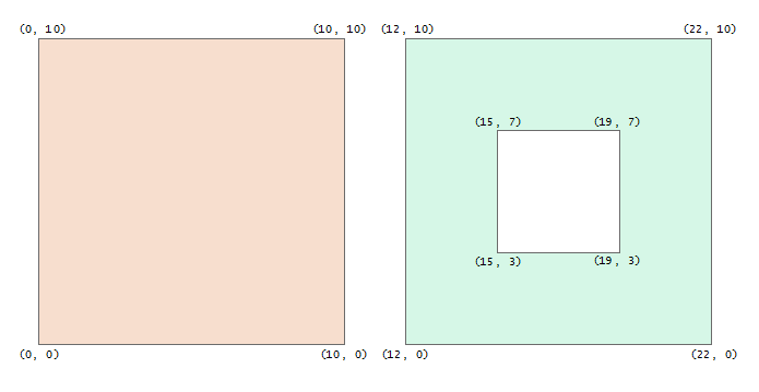
The issue I ran into can be demonstrated by two square polygons, one of which has a hole in it:

arcmap_two_polygons_with_hole_labeled.png

>>> # Create the 2 polygons
>>> poly = arcpy.FromWKT('POLYGON((0 0, 10 0, 10 10, 0 10, 0 0))')
>>> poly_hole = arcpy.FromWKT('POLYGON((12 0, 22 0, 22 10, 12 10, 12 0),'
...                                   '(15 3, 15 7, 19 7, 19 3, 15 3))')
...                                   
>>> # Check the number of parts
>>> poly.partCount
1
>>> poly_hole.partCount
1
>>> 
>>> # Check the multipart property
>>> poly.isMultipart
False
>>> poly_hole.isMultipart
True
>>>

Wait a second, something doesn't add up here.  Both polygons have 1 part, but the polygon with a hole in it is a multipart?  It seems we are witnessing the multi-part single-part polygon, a sideshow favorite that you don't even have to visit the circus to see.

The facile explanation is that the polygon with a hole in it is a multipart because it has an exterior and interior boundary, as opposed to the other polygon that only has an exterior boundary.  Multiple parts, see, simple.  The explanation does make sense, but it also implies that partCount has been broken since ArcGIS 10.0.  Well, maybe partCount has been working all along and the documentation has been wrong for 6 years.  Then again, maybe isMultipart has been broken for 6 years.  Who knows, not me, but I just can't believe I haven't been bitten by this bug long before now.

In terms of what next, assuming Esri Development acknowledges this is either a software or documentation bug, my money is on the documentation getting updated, eventually.  It is always easier to add additional footnotes and asterisks to documentation than it is to update code.  That said, I think there is actually a larger problem with the ArcPy Geometry classes.

I spent some time trying the example above in different spatial systems, even other Esri software components outside of ArcPy, and I have come to the conclusion the real problem is in the labels themselves.  Specifically, the problem lies in the use of "part" to talk about geometries.  Take a look at the List of SQL functions for Esri's ST_Geometry data type, the OGC Methods on Geometry Instances for Microsoft's geometry data type, or the PostGIS Reference; you will not find a single function, method, or property with the word "part" in it.  There are accessor functions for counting geometries, but they count "geometries" and not "parts."  There are accessor functions for counting interior rings, but they count "interior rings" and not "parts."  You see where this is going.

The problem with the ArcPy Geometry classes, at least one of them, is that Esri replaced multiple, specific geometry components with a single generic one, the "part."  By abstracting geometries and rings with parts, not only did they deviate from geospatial standards and norms, they created the sideshow-worthy multi-part single-part polygon.

more
3 2 3,129
JoshuaBixby
MVP Esteemed Contributor

This is the third in a multi-part series on ArcPy cursors; particularly, working with ArcPy cursors as iterable objects in Python.  The first part in the series looks at some of the important components of iteration in Python.  The second part in the series looks at iterating and looping over ArcPy Data Access cursors.  The third part in the series looks at using several Python built-in and itertool functions with ArcPy Data Access cursors.  The fourth part in the series will look at using generators or generator expressions to separate selection or filtering logic for code re-use.  Fifth or following parts are unknown at this point.

The first two parts in this series cover iteration components of Python and iterating/looping in Python, both of which are crucial to understanding and working with iterables.  Beyond manually iterating or looping over an iterable, there are numerous Python built-in functions that work with iterables and sequences.  Starting back in version 2.3, an itertools module was introduced that contains "functions creating iterators for efficient looping."

The focus of this series is treating ArcPy Data Access cursors as Python iterables.  Like most things in life, there is more than one way to answer a question using ArcGIS, and I want to provide some contrasting examples along with Pythonic examples.  As much as I like writing idiomatic Python, there will be plenty of times when using native geoprocessing tools will outperform straight Python.  Writing fast code is great, but it's a separate discussion for a different day.

There are so many built-in and itertool functions that work with iterables, I can't possibly demonstrate them all, but I will demonstrate a handful to illustrate how such functions work nicely with ArcPy Data Access cursors.  For this and future parts in the series, I will leave the previous examples behind in favor of a real-world dataset that readers can download and experiment with themselves.  Specifically, I will use the USA States layer package included with Esri Data & Maps and available on ArcGIS.com.

The same ArcPy Data Access SearchCursor will be used for most of the examples below:

>>> layer = r'USA States\USA States (below 1:3m)'
>>> fields = ["STATE_ABBR", "SHAPE@AREA", "SUB_REGION", "POP2010"]
>>> cursor = arcpy.da.SearchCursor(layer, fields)
>>>

One question that comes up from time to time in the forums/GeoNet is how to count the number of records in a data set or selection set using cursors:

>>> # Example 1: Get record count using ArcGIS geoprocessing tool
>>> arcpy.GetCount_management(layer)
<Result '52'>
>>>
>>> # Example 2: Get record count using variable as counter
>>> with cursor:
...     i = 0
...     for row in cursor:
...         i = i + 1   # or i += 1
...     print i
...
52
>>>
>>> # Example 3: Get record count using built-in list and len functions
>>> with cursor:
...     print len(list(cursor))
...
52
>>>
>>> # Example 4: Get record count using built-in sum function
>>> with cursor:
...     print sum(1 for row in cursor)
...
52
>>>

Looking over the record counting examples:

  • Example 1 uses ArcGIS's Get Count geoprocessing tool.
    • The Get Count tool retrieves the number of records in a feature class, table, layer, or raster; it does not operate against cursors.  It can also be used in the GUI.
  • Example 2 loops over the cursor using a variable as a counter.
    • A counting loop structure is common across a wide range of programming languages.
  • Example 3 uses built-in list and len functions.
    • The list function converts the entire cursor into a Python list, and the len function returns the length of the list, which corresponds to the number of records in the cursor.
    • Creating a Python list does require copying the entire contents of the cursor into memory, which could become an issue for extremely large data sets.
  • Example 4 uses the built-in sum function along with a generator expression.
    • Using a Python generator expression instead of a list does not copy the entire contents of the cursor into memory.

I included Example 1 because it is the highest performing approach to getting record counts of data sets and selection sets within the ArcGIS framework, but it doesn't deal with a cursor as a Python iterable, which is the focus of this series.  Example 2 is functionally and syntactically correct, although I would argue it isn't the most Pythonic.  Examples 3 and 4 both use Python built-in functions that treat a cursor as an iterable, but it is arguable whether Example 3 or 4 is more Pythonic because each approach has strengths and weaknesses.

Another question that comes up occasionally is how to retrieve a record from a data set based on the minimum or maximum values of one of the fields in the data set.  This next set of examples will retrieve the record/row for the state with the highest population in 2010 (POP2010):

>>> # Retrieve table name for data source of layer
>>> desc = arcpy.Describe(layer)
>>> fc_name = desc.featureClass.baseName
>>>
>>> # Example 5: Get maximum population record using ArcGIS geoprocessing tools
>>> summary_table = arcpy.Statistics_analysis(layer,
...                                           "in_memory/summary_max",
...                                           "POP2010 MAX")
...                                      
>>> arcpy.AddJoin_management(layer,
...                          "POP2010",
...                          summary_table,
...                          "MAX_POP2010",
...                          "KEEP_COMMON")
...                     
>>> joined_fields = [(field if "@" in field else ".".join([fc_name, field]))
...                  for field
...                  in fields]
>>> cursor_sql_join = arcpy.da.SearchCursor(layer, joined_fields)
>>> print next(cursor_sql_join)
(u'CA', 41.639274447708424, u'Pacific', 37253956)
>>> del cursor_sql_join
>>> arcpy.RemoveJoin_management(layer, "summary_max")
<Result 'USA States\\USA States (below 1:3m)'>
>>>
>>> # Example 6: Get maximum population record using SQL subquery
>>> sql = "POP2010 IN ((SELECT MAX(POP2010) FROM {}))".format(fc_name)
>>> cursor_sql_subqry = arcpy.da.SearchCursor(layer, fields, sql)                                
>>> print next(cursor_sql_subqry)
(u'CA', 41.639274447708424, u'Pacific', 37253956)
>>> del cursor_sql_subqry
>>>
>>> # Example 7: Get maximum population record by looping and comparing
>>> with cursor:
...     max_row = next(cursor)
...     for row in cursor:
...         if row[3] > max_row[3]:
...             max_row = row
...        
>>> print max_row
(u'CA', 41.639274447708424, u'Pacific', 37253956)
>>>
>>> # Example 8: Get maximum population record using built-in max function
>>> from operator import itemgetter
>>> with cursor:
...     print max(cursor, key=itemgetter(3))
...
(u'CA', 41.639274447708424, u'Pacific', 37253956)
>>>

Looking over the maximum record examples:

  • Examples 5 and 6 require the table name for the data source of the layer.
    • The table name was found using the ArcPy Describe function and properties of two different Describe objects (the property lookups were chained together on line 03)
    • Examples 5 and 6 both need the underlying table name but for different reasons.
      • With Example 5, the base table name is needed to re-create the cursor after the summary statistics table is joined to the layer's source table.
      • With Example 6, the base table name is needed to create the subquery used in the cursor's SQL WHERE clause.
  • Example 5 uses ArcGIS's Summary Statistics and Add Join geoprocessing tools.
    • The Summary Statistics tool finds the maximum population value in the dataset.  The Add Join tool allows the result of the Summary Statistics tool to be linked back to the original layer to find the corresponding record with the maximum population.
    • Before creating a cursor against the newly joined layer, the original fields need to be updated to prepend the table name to the field name (line 16).
  • Example 6 uses an SQL subquery in the WHERE clause of the SQL query.
    • The SQL subquery identifies the maximum population value.  The value(s) returned from the SQL subquery are used to select record(s) in the original data set.
  • Example 7 loops over the cursor using a variable to hold the record with the maximum value.
    • A loop structure is common across a wide range of programming languages.
  • Example 8 uses the built-in max function along with the operator.itemgetter function.
    • The max function operates on an iterable, but it is necessary to use operator.itemgetter since the cursor represents an iterable of tuples and not an iterable of numeric data types.

I included Example 5 because it only uses ArcGIS geoprocessing tools and can be implemented in the GUI.  Although it can be implemented in the GUI with no scripting skills, Example 5 is also the most cumbersome, i.e., it has the most steps, is the slowest, and creates intermediate products.  With just a little bit of SQL or Python knowledge, the doors open to more eloquent and higher performing approaches.  Similar to Example 2 above, Example 7 is functionally and syntactically correct, although I would argue Example 8 is more Pythonic.

Instead of getting just the State with the largest population in 2010, let's print States and their populations by descending population:

>>> # Example 9: Print State and population by descending population
>>> #            using Sort geoprocessing tool
>>> sorted_table = arcpy.Sort_management(layer,
...                                      "in_memory/sorted_pop",
...                                      "POP2010 DESCENDING")
...                                      
>>> cursor_sorted_table = arcpy.da.SearchCursor(sorted_table, fields)
>>> with cursor_sorted_table:
...     for state, area, sub_region, pop2010 in cursor_sorted_table:
...         print "{}, {}".format(state, pop2010)
...         
CA, 37253956
TX, 25145561
NY, 19378102
...
DC, 601723
WY, 563626
PR, -99
>>> del cursor_sorted_table
>>> 
>>> # Example 10: Print State and population by descending population
>>> #             appending SQL ORDER BY clause
>>> sql = "ORDER BY POP2010 DESC"
>>> cursor_orderby_sql = arcpy.da.SearchCursor(layer, fields, sql_clause=(None, sql))
>>> with cursor_orderby_sql:
...     for state, area, sub_region, pop2010 in cursor_orderby_sql:
...         print "{}, {}".format(state, pop2010)
...         
CA, 37253956
TX, 25145561
NY, 19378102
...
DC, 601723
WY, 563626
PR, -99
>>> del cursor_orderby_sql
>>> 
>>> # Example 11: Print State and population by descending population
>>> #             using built-in sorted function
>>> with cursor:
...     for state, area, sub_region, pop2010 in sorted(cursor,
...                                                    key=itemgetter(3),
...                                                    reverse=True):
...         print "{}, {}".format(state, pop2010)
...         
CA, 37253956
TX, 25145561
NY, 19378102
....
DC, 601723
WY, 563626
PR, -99
>>>

Looking over the descending population examples:

  • Example 9 uses ArcGIS's Sort goeprocessing tool.
    • The Sort tool sorts the original table into a new table.  A new cursor needs to be defined using the newly sorted feature class.
  • Example 10 uses an SQL ORDER BY clause.
    • The SQL ORDER BY clause is passed as part of the sql_clause while creating a new cursor.
  • Example 11 uses the built-in sorted function along with the operator.itemgetter function.
    • The sorted function operates on an iterable, but it is necessary to use operator.itemgetter since the cursor represents an iterable of tuples and not an iterable of numeric data types.
    • The sorted function converts the entire cursor into a Python list, and creating a Python list does require copying the entire contents of the cursor into memory, which could become an issue for extremely large data sets.

I included Example 9 because it uses ArcGIS geoprocessing tools and can be implemented easily in the GUI.  Similar to Example 5 above, Example 9 is cumbersome if one is scripting instead of using the GUI.  Example 10 uses some basic SQL for a straightforward solution, although it does involve having to create another cursor instead of recycling the existing cursor.  Example 11 is idiomatic in that it uses the built-in sorted function and treats the cursor as an iterable.  Since sorted does return a newly sorted Python list from an iterable, using the function could become an issue with extremely large data sets.

There are numerous other examples I thought up, but this post is already longer than I expected.  I believe the 3 sets of examples above demonstrate how Python built-in functions that operate on iterables can be used with ArcPy Data Access cursors to write idiomatic Python for ArcGIS.  The next part of the series looks at using generators and generator expressions with ArcPy Data Access cursors.

more
5 2 3,402
JoshuaBixby
MVP Esteemed Contributor

This is the second in a multi-part series on ArcPy cursors; particularly, working with ArcPy cursors as iterable objects in Python.  The first part in the series looks at some of the important components of iteration in Python.  The second part in the series looks at iterating and looping over ArcPy Data Access cursors.  The third part in the series looks at using several Python built-in and itertool functions with ArcPy Data Access cursors.  The fourth part in the series will look at using generators or generator expressions to separate selection or filtering logic for code re-use.  Fifth or following parts are unknown at this point.

The first part in this series is likely a bit academic for some ArcPy scripters, but I believe a little theory goes a long ways to understanding the practice of something, in this case working with ArcPy Data Access cursors in an idiomatic way.  Also, the terms and concepts laid out in the first post will come up time and again throughout the series.

Before moving on, I will put a plug in for a presentation from a few years back: Loop Like A NativeNed Batchelder gives a nice overview of looping in Python, especially for those with looping experience in other programming languages.  It took me several times of watching it for the whole presentation to sink in, but it really did change the way I view iterating and looping in Python.

Recycling the Python list and ArcPy cursor examples from the previous post, let's call iter() to return an iterator for manually stepping through each iterable.

>>> #create list, attach 2 iterators, and retrieve values by
>>> #    calling next() and object.next()
>>> l = [10, 20, 30, 40, 50]
>>> it_l = iter(l)
>>> it2_l = iter(l)
>>> print next(it_l), next(it2_l)
10 10
>>> print it_l.next(), it2_l.next()
20 20
>>> 
>>> #create search cursor, attach 2 iterators, and retrieve values by
>>> #    calling next and object.next()
>>> cur = arcpy.da.SearchCursor(fc, ["OID@", "SHAPE@"])
>>> it_cur = iter(cur)
>>> it2_cur = iter(cur)
>>> print next(it_cur), next(it2_cur)
(1, <Polyline object at 0x1100fcf0[0x1100ff20]>) (2, <Polyline object at 0x1100fcf0[0x1100ff20]>)
>>> print it_cur.next(), it2_cur.next()
(3, <Polyline object at 0x1100fcf0[0x1100ff20]>) (4, <Polyline object at 0x1100fcf0[0x1100ff20]>)
>>> print next(cur)
(5, <Polyline object at 0x1100fcf0[0x1100ff20]>)
>>>

There is a fair amount to comment on with the code above:

  • A single iterable can have multiple iterators simultaneously accessing it.  How the iterable behaves with multiple iterators is implementation specific.
    • As the iterator definition states in the Python Glossary, a list "produces a fresh new iterator each time you pass it to a iter() function or use it in a for loop."  This explains why lines 06-07 and 08-09 are printing out the same values for both iterators.
    • In contrast to the Python list, the ArcPy Data Access search cursor does not produce a new iterator, i.e., each subsequent call to an iter() function returns the same iterator object that is already in use.  In these types of situations, each call to next() moves the iterator ahead one element regardless of which iterator makes the call.  This explains why lines 16-17 show the first and second OID instead of showing the first OID twice.
  • An iterator can be moved ahead by using either the built-in next() function or the object's next method.  Starting at Python 3.0, with the adoption of PEP 3114, the preferred method to manually iterate is the built-in next() function.
  • Since ArcPy Data Access cursors are their own iterator, one doesn't need to call iter() to get an iterator object before calling next().  Line 20 shows the cursor object itself can be passed to next() to retrieve the next item and move the cursor ahead.

Fortunately for us, the Python for statement does a lot of lifting to streamline the steps so we don't have to manually retrieve an iterator and call next() until the end of the iterable is reached.

Revisiting the SearchCursor documentation:

Summary

SearchCursor establishes read-only access to the records returned from a feature class or table.

Returns an iterator of tuples. The order of values in the tuple matches the order of fields specified by the field_names argument.

Discussion

Geometry properties can be accessed by specifying the token SHAPE@ in the list of fields.

Search cursors can be iterated using a For loop.  [Removed at 10.3.1Search cursors also support With statements; using a With statement will guarantee close and release of database locks and reset iteration].

As one can see, the documentation clearly states the arcpy.da.SearchCursor returns an iterator, an iterator of tuples to be specific.  It makes sense to have it return tuples versus lists since we are using a search cursor that can't update data and tuples are immutable by design.  The second statement in the Discussion section is redundant since for in Python iterates over any iterable, SearchCursor or otherwise, but that statement wouldn't stand out as being redundant if Esri didn't remove the rest of the paragraph that used to follow.

This is a not-so quick aside on an Esri #fail, an example of how not to handle customer feedback.

As shown above, prior to ArcGIS 10.3.1, Esri included a couple statements regarding Python with statements.  The fact that ArcPy Data Access cursors support with statements is worth pointing out, even documenting one might say.  The issue with the two statements was really just an issue with the latter statement, I guarantee it!  Guarantee is a strong word, a definitive word, and the problem is not all database locks are closed and released.

A bug was submitted for the documentation to be updated, BUG-000083762: In each cursor documentation, specify the type of lock being closed and released, as a shared lock is still present in the geodatabase after the 'with' statement executes.  The issue was identified as "fixed" in ArcGIS 10.3.1.  If you want to go find that clarification on locks, I already showed it to you.  Yep, there isn't any, they simply removed the statement about locks.  The insult to injury, they also removed a very important statement about Data Access cursors supporting the Python with statement.

Although the documentation speaks to iterators and iterating, I feel a real opportunity was lost with the code samples to demonstrate a handy Python feature.  A lot of ArcGIS users that are new to Python learn the language by emulating code examples.  In terms of showing Pythonic examples, the ArcPy Data Access cursors are a mixed bag.

Code Sample

SearchCursor example 1

Use SearchCursor to step through a feature class and print specific field values and the x,y coordinates of the point.

import arcpy

fc = 'c:/data/base.gdb/well'
fields = ['WELL_ID', 'WELL_TYPE', 'SHAPE@XY']

# For each row print the WELL_ID and WELL_TYPE fields, and the
# the feature's x,y coordinates
with arcpy.da.SearchCursor(fc, fields) as cursor:
    for row in cursor:
        print('{0}, {1}, {2}'.format(row[0], row[1], row[2]))

As pointed out in my earlier soapbox/aside, the ArcPy Data Access documentation fails to mention that cursors support the Python with statement.  That said, support is implied by the use of Python with statements in the examples.  It is worth one's time to read up on Python with statements, and I encourage their use with ArcPy Data Access cursors whenever possible.

Whereas the documentation examples demonstrate using Python with statements, even though the documentation itself doesn't state they are supported, the examples do fail to demonstrate the use of iterable or sequence unpacking.  Iterable or sequence unpacking is a great feature of Python, and it can be used to make code much more compact and readable at the same time.  Sequence unpacking is briefly mentioned in the Python documentation for Tuples and Sequences, and PEP 3132 -- Extended Iterable Unpacking discusses changes introduced in Python 3.0.

Let's take a look at how iterable unpacking can be used with SearchCursor example 1 from above.

import arcpy

fc = 'c:/data/base.gdb/well'
fields = ['WELL_ID', 'WELL_TYPE', 'SHAPE@XY'
]

# For each row print the WELL_ID and WELL_TYPE fields, and the
# the feature's x,y coordinates

# Original example using sequence indexing
with arcpy.da.SearchCursor(fc, fields) as cursor:
    for row in cursor:
        print('{0}, {1}, {2}'.format(row[0], row[1], row[2]))

# Example using manual sequence unpacking
with arcpy.da.SearchCursor(fc, fields) as cursor:
    for row in cursor:
        well_id = row[0]
        well_type = row[1]
        well_xy = row[2]
        print('{0}, {1}, {2}'.format(well_id, well_type, well_xy))

# Example using built-in sequence unpacking
with arcpy.da.SearchCursor(fc, fields) as cursor:
    for well_id, well_type, well_xy in cursor:
        print('{0}, {1}, {2}'.format(well_id, well_type, well_xy))

I provided an example of manual sequence unpacking because it is fairly common to see that pattern with people coming over to Python from other languages.  Although manual unpacking is syntactically and functionally correct, it can usually be replaced by using built-in unpacking, thus saving some lines of code and being more idiomatic.  With this specific series of examples, it turns out that using built-in sequence unpacking isn't any more compact than using sequence indexing; however, I find reading and maintaining code that uses sequence unpacking is much more straightforward than having to remember which index means what in a sequence.

The Python for statement, with statement, and iterable/sequence unpacking; all essentials when working with the iterable cursor.

more
4 0 5,005
JoshuaBixby
MVP Esteemed Contributor

This is the first in a multi-part series on ArcPy cursors; particularly, working with ArcPy cursors as iterable objects in Python.  The first part in the series looks at some of the important components of iteration in Python.  The second part in the series looks at iterating and looping over ArcPy Data Access cursors.  The third part in the series looks at using several Python built-in and itertool functions with ArcPy Data Access cursors.  The fourth part in the series will look at using generators or generator expressions to separate selection or filtering logic for code re-use.  Fifth or following parts are unknown at this point.

This and the following series of blog posts focuses on ArcPy Data Access cursors in the context of iteration, hence the title of the series.  Now, it might seem silly to talk about iterable cursors since a cursor is basically worthless without iteration, but my experience scripting with ArcPy cursors and with responding to questions on GeoNet has motivated me to share some Pythonic ways of thinking about and working with cursors.

When talking about iteration in Python, there are numerous terms and expressions that can be relevant to a discussion.  Five terms that I believe to be especially important, and relevant to this series of blog posts, are:

Glossary

generator

A function which returns an iterator. It looks like a normal function except that it contains yield statements for producing a series of values usable in a for-loop or that can be retrieved one at a time with the next() function. Each yield temporarily suspends processing, remembering the location execution state (including local variables and pending try-statements). When the generator resumes, it picks-up where it left-off (in contrast to functions which start fresh on every invocation).

generator expression

An expression that returns an iterator. It looks like a normal expression followed by a for expression defining a loop variable, range, and an optional if expression. The combined expression generates values for an enclosing function:

>>> sum(i*i for i in range(10))         # sum of squares 0, 1, 4, ... 81
285

iterable

An object capable of returning its members one at a time. Examples of iterables include all sequence types (such as list, str, and tuple) and some non-sequence types like dict and file and objects of any classes you define with an __iter__() or __getitem__() method. Iterables can be used in a for loop and in many other places where a sequence is needed (zip(), map(), ...). When an iterable object is passed as an argument to the built-in function iter(), it returns an iterator for the object. This iterator is good for one pass over the set of values. When using iterables, it is usually not necessary to call iter() or deal with iterator objects yourself. The for statement does that automatically for you, creating a temporary unnamed variable to hold the iterator for the duration of the loop. See also iterator, sequence, and generator.

iterator

An object representing a stream of data. Repeated calls to the iterator’s next() method return successive items in the stream. When no more data are available a StopIteration exception is raised instead. At this point, the iterator object is exhausted and any further calls to its next() method just raise StopIteration again. Iterators are required to have an __iter__() method that returns the iterator object itself so every iterator is also iterable and may be used in most places where other iterables are accepted. One notable exception is code which attempts multiple iteration passes. A container object (such as a list) produces a fresh new iterator each time you pass it to the iter() function or use it in a for loop. Attempting this with an iterator will just return the same exhausted iterator object used in the previous iteration pass, making it appear like an empty container.

sequence

An iterable which supports efficient element access using integer indices via the __getitem__() special method and defines a len() method that returns the length of the sequence. Some built-in sequence types are list, str, tuple, and unicode. Note that dict also supports __getitem__() and __len__(), but is considered a mapping rather than a sequence because the lookups use arbitrary immutable keys rather than integers.

Compared to the old glossary from ArcGIS Resources, now renamed GIS Dictionary and housed over at Esri Support, the Python Glossary is quite substantial.  That said, the Python Glossary is also one of those that makes sense to people that already know the answer, but it can be a bit of a reach for people new to the language.

From looking over the glossary excerpt above, one can tease out that a few special/magic/dunder methods are very important to iteration:  __iter__(), __getitem__(), and next() (or __next__() if one is working in Python 3.x).  There are also a couple of important built-in functions that interact with those methods:  iter() and next().  And last but not least, the for loop and the yield statement.  There are more methods, functions, statements, and control structures involved with iteration, but the aforementioned ones are central to any discussion.  For those readers interested in learning more about iterators, generators, sequences, etc...; there are numerous primers and tutorials that have already been written and are just a quick Google search away.

Lists are so common in Python, and newcomers to the language get exposure to them so early, that I will use Python list examples for context alongside the ArcPy Data Access search cursor examples.  The Python Glossary states that a list is "a built-in Python sequence," and a sequence is "an iterable which supports efficient element access using integer indices...."  The ArcPy Data Access SearchCursor documentation states the search cursor "returns an iterator of tuples."  Since iterators are also iterable, one gets a sense that built-in functions and expressions commonly used for manipulating lists may also be used with ArcPy cursors.

Although one can use the built-in dir() function to attempt to return a list of valid attributes for an object, I am going to forgo inspecting the objects that way because it will introduce clutter from all of the attributes that aren't related to iteration.  Instead, I will rely on the built-in isinstance() function along with built-in abstract base classes (ABCs) to look at iteration traits.

>>> #import relevant ABCs from collections module
>>> from collections import Iterable, Iterator, Sequence
>>> 
>>> #create a sample list and arcpy.da.SearchCursor
>>> l = [10, 20, 30, 40, 50]
>>> cur = arcpy.da.SearchCursor(fc,["OID@", "SHAPE@"])
>>> 
>>> #look at iteration traits of sample objects
>>> abcs = (Iterable, Iterator, Sequence)
>>> [isinstance(l, abc) for abc in abcs]
[True, False, True]  #Iterable, not Iterator, Sequence
>>>
>>> [isinstance(cur, abc) for abc in abcs]
[True, True, False]  #Iterable, Iterator, not Sequence
>>> 
>>> #look at the types for sample objects and iterators of sample objects
>>> it_l = iter(l)
>>> type(l)
<type 'list'>
>>> type(it_l)
<type 'listiterator'>
>>> 
>>> it_cur = iter(cur)
>>> type(cur)
<type 'da.SearchCursor'>
>>> type(it_cur)
<type 'da.SearchCursor'>
>>> 
>>> #look at identify of cursor objects
>>> id(cur)
262686224
>>> id(it_cur)
262686224
>>>

As one can see above, which basically demonstrates what is stated in the Python Glossary, a list is both an iterable and sequence but not an iterator whereas an ArcPy Data Access search cursor is both an iterable and iterator but not a sequence.  From lines 20-21, we see that calling iter() on a list returns a new type of object as well as a new object, i.e., the listiterator.  From lines 26-27, we see that calling iter() on a search cursor returns a search cursor instead of a new iterator object.  Not only is a search cursor returned by calling iter(), but lines 30-33 show that the same search cursor object is returned when doing so.  This design pattern of having an iterable be its own iterator is fairly common in Python.

In the next post in this series, we will move beyond the components of iteration and start actually iterating over Python objects, including ArcPy Data Access cursors.

more
3 0 3,588
63 Subscribers