- Home
- :
- All Communities
- :
- Products
- :
- ArcGIS Spatial Analyst
- :
- ArcGIS Spatial Analyst Questions
- :
- Principal Components: what do they mean?
- Subscribe to RSS Feed
- Mark Topic as New
- Mark Topic as Read
- Float this Topic for Current User
- Bookmark
- Subscribe
- Mute
- Printer Friendly Page
- Mark as New
- Bookmark
- Subscribe
- Mute
- Subscribe to RSS Feed
- Permalink
- Report Inappropriate Content
Hi -
I understand that principle components are calculated such that the first explains the greatest amount of variation in a dataset, the second PC explains the greatest amount of remaining variation, and so on. I understand PCs are uncorrelated variables that retain information in the original dataset using reduced dimensions.
What I'm unclear on is what PCs mean in terms of the multiband raster output from the Principal Components tool. I can look at my Eigenvalues for each PC and determine how many to use to maintain the variation in my dataset, but I don't know how to interpret the PCs in raster form.
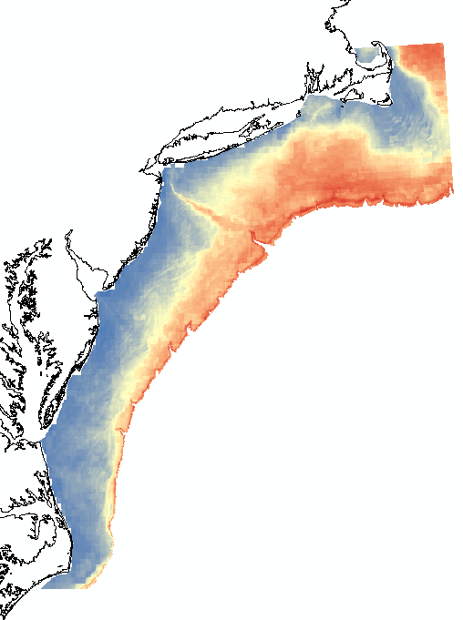
For example, here is PC1, with values ranging from 4.6 (red) to 0 (blue). What do these values mean? My best guess is that these values are 'distances' or errors from the PC1 axis.
Solved! Go to Solution.
Accepted Solutions
- Mark as New
- Bookmark
- Subscribe
- Mute
- Subscribe to RSS Feed
- Permalink
- Report Inappropriate Content
Hi Heather
The PCA summarises all of your data into the new axes that best explain the
variation found in your data set, with most of the variation being
explained in the first few axes (you probably already know all that).
But to figure out what the various axes actually represent, relating back
to your input raters, then I find it very useful to run the Band Collection
Statistics tool (Spatial Analyst Tools/Multivariate/Band Collection
Statistics).
For your input raster bands, add both your PCA exes and the various raster
bands that were used to create the PCA axes, and make sure to tick the
"Compute covariance and correlation matrices" tick-box. This will then
create a statistics text file where it calculates the correlation between
each of the PCA axes and the various raster files used as input (both
positive and negative correlations). So, for example, it will show that
altitude may have a correlation value of 0.99, mintempcoldmonth 0.90,
maxtempwarmmonth 0.91, etc.(this is from a real example) with PCA axis 2.
The input variables used in this example are inherently correlated as
temperature decreases with altitude and the PCA has nicely distilled all of
this this variation into a single axis.
So then you know what the pixels represent when interpreting your analysis.
Lastly, PCA needs to standardize the input variables so that it can compare
apples with apples, and so analyse altitude, rainfall, temperature,
vegetation indices, clay percentage, etc.(all which are corded on different
scales) into one PCA analysis.
I hope this helps.
Regards
Mervyn
- Mark as New
- Bookmark
- Subscribe
- Mute
- Subscribe to RSS Feed
- Permalink
- Report Inappropriate Content
I don't have an answer, but wanted to post this here for others who may be curious about the subject and how it relates to image compression. The Nixon/Elvis example is interesting.
Principle Components and Imagery - Simon Jackman.
Chris Donohue, GISP
- Mark as New
- Bookmark
- Subscribe
- Mute
- Subscribe to RSS Feed
- Permalink
- Report Inappropriate Content
Heather,
your our understanding of PC analysis is on the mark. The resultant bands the directions in the data where there exists the most variance, where the data is most spread out. The question of what the actual values mean though is something a little more complex. Rather than try and explain it in a few brief sentences here the is a good reference which lays out the analysis and what the values mean found here
i hope this helps
Gordon
- Mark as New
- Bookmark
- Subscribe
- Mute
- Subscribe to RSS Feed
- Permalink
- Report Inappropriate Content
Hi Gordon,
Thanks - that is a great link to a very clear and concise explanation of a PCA analysis. But I still don't understand what the raster PC pixel values are, or how they are calculated. PC1 is an axis along the direction of greatest variance (side question: because I'm working with spatial data, are directions true directions; e.g. the direction of greatest variance denoted by PC1 above is inshore -> offshore?), but what does a high pixel value mean vs. a low pixel value?
If I were to hazard another guess following: pca - What are principal component scores? - Cross Validated , I'd guess that each pixel value is a PC score. In other words, a given pixel(x)'s value in PC1 is a linear recombination calculated as the product of var1 at pixel(x) * var1 loading for PC1 and then summed across all variables at pixel(x).
Following this logic, a pixel w a high value in PC1 likely had original variables with high values that loaded heavily in PC1 (because multiple sums of a big variable value * a high loading would lead to larger numbers). So I guess I would interpret PC1 as representing original variables that were generally low valued inshore, and high valued offshore.
Am I on the right track?
And if so, it begs a follow up question: why are none of the PC1 raster pixel values negative? A given variable can load negatively w a given PC: if linear recombination is how pixel values are calculated, some could be less than zero. Does Arc include some sort of standardization in the calculation?
- Mark as New
- Bookmark
- Subscribe
- Mute
- Subscribe to RSS Feed
- Permalink
- Report Inappropriate Content
Hi Heather
The PCA summarises all of your data into the new axes that best explain the
variation found in your data set, with most of the variation being
explained in the first few axes (you probably already know all that).
But to figure out what the various axes actually represent, relating back
to your input raters, then I find it very useful to run the Band Collection
Statistics tool (Spatial Analyst Tools/Multivariate/Band Collection
Statistics).
For your input raster bands, add both your PCA exes and the various raster
bands that were used to create the PCA axes, and make sure to tick the
"Compute covariance and correlation matrices" tick-box. This will then
create a statistics text file where it calculates the correlation between
each of the PCA axes and the various raster files used as input (both
positive and negative correlations). So, for example, it will show that
altitude may have a correlation value of 0.99, mintempcoldmonth 0.90,
maxtempwarmmonth 0.91, etc.(this is from a real example) with PCA axis 2.
The input variables used in this example are inherently correlated as
temperature decreases with altitude and the PCA has nicely distilled all of
this this variation into a single axis.
So then you know what the pixels represent when interpreting your analysis.
Lastly, PCA needs to standardize the input variables so that it can compare
apples with apples, and so analyse altitude, rainfall, temperature,
vegetation indices, clay percentage, etc.(all which are corded on different
scales) into one PCA analysis.
I hope this helps.
Regards
Mervyn
- Mark as New
- Bookmark
- Subscribe
- Mute
- Subscribe to RSS Feed
- Permalink
- Report Inappropriate Content
Hi Mervyn,
Thanks for your answer. I arrived at a similar conclusion using different methods, but would like to put it to the group to see if others find it plausible.
My understanding is that the variation in layers that load heavily with a given PC; i.e. layers that have high positive or low negative eigenvectors, is captured by the given PC. Layers with high positive eigenvectors are directly related to the PC; layers with low negative eigenvectors are inversely related. For a given PC, a high pixel is a location where layers with high positive eigenvectors also had high values (direct relationship). A low pixel is a location where layers with low negative eigenvectors has high values (inverse relationship).
I tested this by running a PCA on a very small number of input layers so I could easily observe the relationships between inputs and PCs, and it holds true.
Does anyone see any flaws in this conclusion?