Ripley's K Confidence Envelope doesn't follow the blue expected line

[Mareike_TabeaScheller]

Hello!
I'm working for the first time with the Spatial Statistics tools.
I have point data of birds on an island. I want to calculate the K-Function, but the result graph always shows a Confidence Envelope that is under the blue expected line. Why is that? Shouldn't the confidence envelope follow the expected line?
I would be glad if anyone had a suggestion what mistake I might have made here.

Mareike

[LaurenceCulot]

Thanks. I understand what the L transformation does, so if that is indeed the formula that is being used then it seems like the output.dbf should describe the fields as ExpectedL(Distance) and ObservedL rather than saying K. The .dbf fields differ from the results window box, which labels the output fields Distance and L(d).

My reading on the L transformation suggests that it is used to make graphical interpretation of results more straightforward. In that case, it would be more helpful if the graphical output displayed L(d)-d on the y axis so that the expected line (which from my understanding represents complete spatial randomness) is equal to y=0 rather than a line with a slope of 1. Also, the legend of the graphic should say ExpectedL and ObservedL to be consistent with the formula that is used.

I look forward to hearing your response for why the confidence intervals at some distances do not include the expected value for L (CSR).

I have exactly the same problem with the Ripley's k function confidence envelope. I tried to run the analysis with and without edge correction but always obtained a confidence envelope going below the expected line from some distance. Is there a response/solution for this problem?

[LaurenScott]

Hi Laurence,
Thanks for your question.  There are a couple different reasons that the confidence envelope may not follow the expected line.

1) Differences between weighted and unweighted K function.

When you run K function just on your point features (no weight field), the confidence envelope will tend to follow the Expected Blue line.  The confidence envelope is created by taking your point features and (conceptually) throwing them down into your study area (a rectangle if you select minimum enclosing rectangle, otherwise the polygon feature you provide).  It repeats this random process of throwing down your points, letting them fall where they may within the study area, for 9, 99, or 999 times.  Each time it computes the K function value for all distances and the lower confidence line is derived from the lowest observed L(d) values; the upper confidence line is derived from the largest L(d) values.  If the study area is simple (rectangle, circle), the confidence envelope will enclose the expected line (but see #2 and #3 below).

When you run the K function with a Weight Field, the confidence envelope will tend to follow the Observed L(d) line (the red line).  In this case the confidence envelope is created by throwing down the feature values (the weights) onto the existing feature locations.  The locations themselves remain fixed, only the weights associated with the features are randomly re-distributed for 9, 99, or 999 permutations.  Because the spatial distribution of your points restrict where the values can land, the confidence envelope follows the observed L(d) line showing you the range of outcomes given the fixed location of your features.

2) Boundary correction.

The K function works by counting all feature pairs within a given distance of each feature.  When you specify NONE for the Boundary Correction method, this counting process is biased near the edges/boundaries.  Imagine a circle representing the distance where pairs will be counted.  When that circle overlays a point/feature near an edge, a portion of the circle will fall outside the study area where there are no points.... the counts will be smaller because there are fewer pairs within the circle.  If there really are no points/features outside the study area, this drop in clustering at increasing distances is valid.  If the boundaries are an artifact, you should correct for this undercounting bias by selecting a Boundary Correction method.

3) Study area size.

The K Function is one of two tools in the Spatial Statistics Toolbox that is VERY (VERY) sensitive to study area size (the other tool is Average Nearest Neighbor).  Imagine a cluster of points enclosed by a very, very tight study area... with that configuration, the pattern appears dispersed.  Now imagine that same cluster of points enclose by a very large study area (so the cluster is at the middle with vast space all around it)... now the points would definitely appear clustered.  For a graphic, please see: http://help.arcgis.com/en/arcgisdesktop/10.0/help/index.html#/Multi_Distance_Spatial_Cluster_Analysi... (About the 12th usage tip that starts: "The k-function statistic is very sensitive to the size of the study area.").

4) Study area shape.

In #1 above, I described how the confidence envelopes are constructed.  In essence, features are pitched onto your study area, each feature landing where it may.  When you have a very convoluted study area, this can impact where features are allowed to land.  Hmmm... okay imagine a square study area with two long skinny arms, two long skinny legs, and a head 🙂  Features that fall into the arms and legs will have fewer neighbors because the study area itself doesn't allow many features to fall into the skinny parts... (does that make sense)? 

But this kind of thing can also happen if you elect the Minimum Enclosing Rectangle study area when your features aren't very rectangular.  Imagine a set of features randomly distributed into a circle.  Then imagine a rectangular study area around it.  In the corners of the study area there will be no features.  When the K function starts counting pairs near those corners, the pair counts will drop.  This can result in a drooping confidence envelope for weighted K function.

I hope this helps.  If you still have questions, please feel free to contact me.  I am happy to look at your data and evaluate the results to see why you might be seeing the drooping confidence envelope even when you apply a boundary correction method.

Best wishes,
Lauren

Lauren M Scott, PhD
Esri
Geoprocessing, Spatial Statistics
LScott@esri.com

[LaurenScott]

A bit more... we have identified a bug in the Multi-Distance Spatial Cluster Analysis (Ripley's K Function) tool, for ArcGIS 10.0 only, when you select Simulate Outer Boundary Values for the Boundary Correction method and also elect to Compute a Confidence Envelope (sorry!). In this circumstance, you will notice that the observed L(d) values (the red line on the K Function graph) will have the appropriate (accurate) correction, but that the confidence envelope lines (the gray lines on the graph) will continue to droop because no correction is applied. I'm very sorry that we didn't catch this problem sooner!

Fortunately, since almost all of the tools in the Spatial Statistics toolbox are written using Python, you have our source code and can correct the bug if you so choose. Below are instructions for making the correction (it involves changing one word in the source code). If you are not comfortable making this change, but need this fix, please contact me and I'm happy to send you the corrected Python script file.

To make the correction yourself:
1) Navigate to the Scripts folder and locate the KFunction.py script: <ArcGIS>\Desktop10.0\ArcToolbox\Scripts
2) Create a backup copy of this script file (name the copy something like KFunctionSave.py)... this is just in case something goes wrong.
3) Open KFunction.py with any text editor (like Notepad, for example). Alternatively, from within ArcMap you can also just right click on the K Function tool (via the Catalog or the ArcToolbox pane) and select Edit to access the source code.
4) Locate the following section of code (at about line 517) and make the change indicated below (shown in red):

#### Resolve Simulate Points ####
if self.simulate:
[INDENT]simTable = GAPY.ga_table()
tempN = len(newTable)
simID = self.maxID + 1
for i in xrange(tempN):
[INDENT]row = newTable
id = row[0]
x,y = row[1]
simTable.insert(id, (x,y), 1.0)
if near[id] <= self.stepMax:
[INDENT]nearX, nearY = nearXY[id]
dX = nearX + (nearX - x)
dY = nearY + (nearY - y)
point = (dX, dY)
inside = UTILS.pointInPoly(point, self.studyAreaPoly, tolerance = self.tolerance)
if not inside:
[INDENT]newTable.insert(simID, point, 1.0) <-- change "newTable" to "simTable" on this line: simTable.insert(simID, point, 1.0)
newSimDict[simID] = id
simID += 1
[/INDENT][/INDENT][/INDENT][/INDENT]


Again, my sincere apologies for this error. Please contact me (or contact Tech Support) if you have any questions or concerns.
Lauren

Lauren M Scott, PhD
Esri
Geoprocessing, Spatial Statistics
LScott@Esri.com

[VitaBakker]

Has this issue been resolved? When I apply Ripley's K, I simulate outer boundaries and have a polygon, and the study area is a feature class. The upper and lower confidence level lines still don't follow the expected K. 

Best, 

Vita 

[VladimirLisitsin]

Hi Laurence,
Thanks for your question.  There are a couple different reasons that the confidence envelope may not follow the expected line.

1) Differences between weighted and unweighted K function.

When you run K function just on your point features (no weight field), the confidence envelope will tend to follow the Expected Blue line.  The confidence envelope is created by taking your point features and (conceptually) throwing them down into your study area (a rectangle if you select minimum enclosing rectangle, otherwise the polygon feature you provide).  It repeats this random process of throwing down your points, letting them fall where they may within the study area, for 9, 99, or 999 times.  Each time it computes the K function value for all distances and the lower confidence line is derived from the lowest observed L(d) values; the upper confidence line is derived from the largest L(d) values.  If the study area is simple (rectangle, circle), the confidence envelope will enclose the expected line (but see #2 and #3 below).

When you run the K function with a Weight Field, the confidence envelope will tend to follow the Observed L(d) line (the red line).  In this case the confidence envelope is created by throwing down the feature values (the weights) onto the existing feature locations.  The locations themselves remain fixed, only the weights associated with the features are randomly re-distributed for 9, 99, or 999 permutations.  Because the spatial distribution of your points restrict where the values can land, the confidence envelope follows the observed L(d) line showing you the range of outcomes given the fixed location of your features.

2) Boundary correction.

The K function works by counting all feature pairs within a given distance of each feature.  When you specify NONE for the Boundary Correction method, this counting process is biased near the edges/boundaries.  Imagine a circle representing the distance where pairs will be counted.  When that circle overlays a point/feature near an edge, a portion of the circle will fall outside the study area where there are no points.... the counts will be smaller because there are fewer pairs within the circle.  If there really are no points/features outside the study area, this drop in clustering at increasing distances is valid.  If the boundaries are an artifact, you should correct for this undercounting bias by selecting a Boundary Correction method.

3) Study area size.

The K Function is one of two tools in the Spatial Statistics Toolbox that is VERY (VERY) sensitive to study area size (the other tool is Average Nearest Neighbor).  Imagine a cluster of points enclosed by a very, very tight study area... with that configuration, the pattern appears dispersed.  Now imagine that same cluster of points enclose by a very large study area (so the cluster is at the middle with vast space all around it)... now the points would definitely appear clustered.  For a graphic, please see: http://help.arcgis.com/en/arcgisdesktop/10.0/help/index.html#/Multi_Distance_Spatial_Cluster_Analysi... (About the 12th usage tip that starts: "The k-function statistic is very sensitive to the size of the study area.").

4) Study area shape.

In #1 above, I described how the confidence envelopes are constructed.  In essence, features are pitched onto your study area, each feature landing where it may.  When you have a very convoluted study area, this can impact where features are allowed to land.  Hmmm... okay imagine a square study area with two long skinny arms, two long skinny legs, and a head 🙂  Features that fall into the arms and legs will have fewer neighbors because the study area itself doesn't allow many features to fall into the skinny parts... (does that make sense)? 

But this kind of thing can also happen if you elect the Minimum Enclosing Rectangle study area when your features aren't very rectangular.  Imagine a set of features randomly distributed into a circle.  Then imagine a rectangular study area around it.  In the corners of the study area there will be no features.  When the K function starts counting pairs near those corners, the pair counts will drop.  This can result in a drooping confidence envelope for weighted K function.

I hope this helps.  If you still have questions, please feel free to contact me.  I am happy to look at your data and evaluate the results to see why you might be seeing the drooping confidence envelope even when you apply a boundary correction method.

Best wishes,
Lauren

Lauren M Scott, PhD
Esri
Geoprocessing, Spatial Statistics
LScott@esri.com

Hi Lauren,

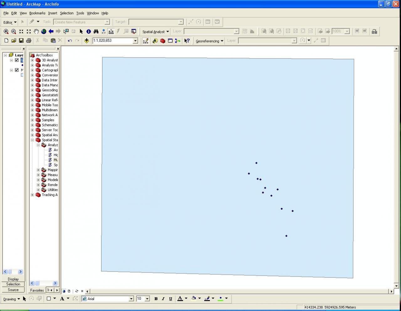
I also have a problem with the Ripley's confidence envelopes, almost regardless of the shape of the study area. It is easier to illustrate by an example. There are 11 points, quite obviously arranged in a band, within a quasi-rectangular study area: [ATTACH=CONFIG]13657[/ATTACH]
On the Ripley's K graph (unweighted, study area defined, 99 permutations; ArcGIS 9.3.1), the observed line plots above the expected line (as expected for a clustered pattern). However, the confidence envelope closely follows the observed line. Curiously, the envelope converges to a single horizontal line which exactly coincides with the expected line at the distance equal to the distance between the furthermost sample points:
[ATTACH=CONFIG]13658[/ATTACH]
This appears to suggest that the permutations are not based on true random sets of points, with each point randomly placed within a study area. The convergence to a horizontal line indicates that the 'random' permutations are reproducing essentially the same pattern, almost precisely maintaining the same maximum point separation. ArcGIS outputs in this example are not due to weighting, or the study area shape or size, or the boundary effects - 999 permutations using a much larger precisely rectangular area with the points in the middle produce the same results. The only way I could coax ArcGIS' Ripley's K function to confirm the existence of statistically significant clustering was by adding one or more 'fake' data points significantly removed from the cluster.

I would appreciate it if you could advise me how to produce more reliable confidence envelopes.

Thank you.

Regards,
Vladimir

[VladimirLisitsin]

Just to clarify the point on the convergence between the confidence envelope and the observed line from the previous post. Theoretically, they should indeed converge at the MAX(L(t)) for a given study area size and the number of points - but only at a distance of at least half of the maximum dimension of the study area. And in cases of geometrically simple study areas and unweighted K simulations, the confidence envelopes should not deviate too much from the Expected line (apart from the usual boundary-effect drop-off at larger distances) �?? as Lauren has repeatedly mentioned. The problem is, unweighted simulations sometimes seem to behave similar to the weighted ones�?�

[LaurenScott]

A bit more again. 
I found another problem in the Ripley�??s K function tool associated with the confidence envelope.  It is most apparent when the study area is much larger than the points being analyzed, but could also show up with the Minimum Enclosing Rectangle option if the distribution of the points is not very rectangular.  Unfortunately, I found this bug too late to get the fix into 10.1 (not yet released) or into 10.0 service pack 5. 

Consequently, I'm attaching a file that fixes this problem for ArcGIS 10.0 (it also fixes the issue described earlier relating to "simTable").  This fix will only work for ArcGIS 10.0.  Here are the instructions for installing the fix:

1) Navigate to your <ArcGIS>\Desktop10.0\ArcToolbox\Scripts folder.
2) Rename the KFunction.py file (to something like KFunctionOrig.py <-- this is just in case �?�)
3) Copy the attached KFunction.py into that same Scripts folder
4) Run the K function as usual.

Please feel free to contact me if you have any questions or concerns.

My sincere apologies,
Lauren

Lauren M. Scott, PhD
LScott@esri.com
Esri
Geoprocessing, Spatial Statistics

[boonejardot]

Yup the tech pretty much nailed it.  Ripleys K and the blue line/ confidence envelope.  This stuff is kind of advanced just so ya know.  The blue line is based on a rectangular area.  Therefore if the study area is not rectangular, I E an Island/Circular jagged etc, the points will only fall within your study area.  therefore the blue line is irrelevant if you are using a confidence envelope.  Run your analysis as if the confidence envelope IS the blue line.  Any divergence from that, shows something that may not be random.

[AprilNewlander1]

I too have been having the same problem with the expected line falling outside the CI.  See attachments... pattern analysis shows the study area and points I am using.  Each point represents a 1x1 m grid cell that contains a 1-4 m plant (classified as 1 for plant size class) as determined by LiDAR data.  The area is divided into 2 study areas: above the road and below the road.  Above unweighted shows results of UW ripley's; the figure Above is the weighted (all weights =1; represent a 1x1 m grid cell that has a plant 1-4 m tall in it) observation plotted with the unweighted CI and the expected line adjusted to zero.  Notice the drooping CI and that the pattern changed dramatically from that of the unweighted observation...from clustered across all distance scales (UW) to small scale clustering and large scale dispersion.  The figure 'below Unweighted' and 'below' show the analysis below the road.  I used the 'simulate outer boundary values' for edge correction; and user defined study area.  I am aware that maybe the study area size could impact my results (clustering is an artifact).  Does the weighted analysis seem appopriate to use to represent the pattern?