- Home
- :
- All Communities
- :
- Industries
- :
- Education
- :
- Education Blog
- :
- Accessing and Using Lidar Data from The National M...
Accessing and Using Lidar Data from The National Map in ArcGIS Pro
- Subscribe to RSS Feed
- Mark as New
- Mark as Read
- Bookmark
- Subscribe
- Printer Friendly Page
In this essay, I will share how to access, use, and analyze Lidar data from The National Map in ArcGIS Pro. By extension it could be applied to Lidar data from other sites as well, but the USGS data portal NationalMap remains an excellent resource for spatial data, and why I focus on it here. For videos of these procedures, go to the YouTube Channel geographyuberalles and search on Lidar. For an entire book with exercises on using Lidar in ArcGIS Pro, see the Esri Press book from two of my favorite colleagues Kathryn Keranen and Bob Kolvoord.
From a user perspective, in my view the National Map site is still a bit challenging, where the user encounters moments in the access and download process where it is not clear how to proceed. However, (1) the site is slowly improving; (2) the site is worth investigating chiefly because of its wealth of data holdings: It is simply too rich of a resource to ignore. One challenging thing about using NationalMap is, like many other data portals, how to effectively narrow the search from the thousands of search results. This in part reflects the open data movement that I have been writing about on the Spatial Reserves data blog, so this is a good problem to have, albeit still cumbersome in this portal. Here are the procedures to access and download the Lidar data from the site:
- To begin: Visit the National Map: https://nationalmap.gov/ > Select “Elevation” from this page.
- Select “Get Elevation Data” from the bottom of the Elevation page. This is one of several quirks about the site – why isn’t this link in a more prominent position or in a bolder font?
- From the Data Elevation Products page left hand column: Select “1 meter DEM.”
- Select the desired format. Select “Show Availability”. Zoom to the desired area using a variety of tools to do so. In my example, I was interested in Lidar data for Grand Junction, in western Colorado.
- Note that the list of available products will appear in the left hand column. Lidar is provided in 10000 x 10000 meter tiles. In my example, 108 products exist for the Grand Junction Lidar dataset. Use “Footprint” to help you identify areas in which you need data–the footprints appear as helpful polygon outlines. At this point, you could save your results as text or CSV, which I found to be quite handy.
- You can select the tiles needed one by one to add to your cart or select “Page” to select all items. Select the Cart where you can download the tiles manually or select the “uGet Instructions” for details about downloading multiple files. Your data will be delivered in a zip format right away, though Lidar files are large and may require some time to download.
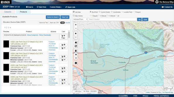
The National Map interface as it appeared when I was selecting my desired area for Lidar data.
Unzip the LAS data for use in your chosen GIS package. To bring the data into ArcGIS Pro, create a new blank project and name it. Then, Go to Analysis > Tools > Create LAS dataset from your unzipped .las file, noting the projection (in this case, UTM) and other metadata. Sometimes you can bring .las files directly into Pro without creating a LAS dataset, but with this NationalMap Lidar data, I found that I needed to create a LAS dataset first.
Then > Insert: New Map > add your LAS dataset to the new map. Zoom in to see the lidar points. View your Lidar data in different ways using the Appearance tab to see it as elevation, slope, aspect (shown below), and contours. Use LAS dataset to raster to convert the Lidar data to a raster. In a similar way, I added the World Hydro layer so I could see the watersheds in this area, and USA detailed streams for the rivers.
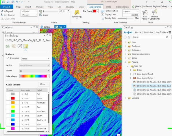
Aspect view generated from Lidar data in ArcGIS Pro.
There are many things you can do with your newly downloaded Lidar data: Let’s explore just a few of those. First, create a Digital Elevation Model (DEM) and a Digital Surface Model (DSM). To do this, in your .lasd LAS dataset > LAS Filters > Filter to ground, and visualize the results, and then use LAS Dataset to Raster, using the Elevation as the value field. Your resulting raster is your digital elevation model (DEM). Next, Filter to first return, and then convert this to a raster: This is your digital surface model (DSM). After clicking on sections of each raster to compare them visually, go one step further and use the Raster Calculator to create a comparison raster: Use the formula: 1streturn_raster – (subtract) the ground_raster. The first return result is essentially showing the objects or features on the surface of the Earth–the difference between “bare earth” elevation and the “first return”–in other words, the buildings, trees, shrubs, and other things human built and natural. Symbolize and classify this comparison surface to more fully understand your vegetation and structures. In my study area, the difference between the DEM and the DSM was much more pronounced on the north (northeast, actually) facing slope, which is where the pinon and juniper trees are growing, as opposed to the barren south (southwest) facing slope which is underlain by Mancos Shale (shown below).

Comparison of DEM and DSM as a “ground cover” raster in ArcGIS Pro.

My photograph of the ridgeline, from just east of the study area, looking northwest. Note the piñon and juniper ground cover on the northeast-facing slopes as opposed to the barren southwest facing slope.
Next, create a Hillshade from your ground raster (DEM) using the hillshade tool. Next, create a slope map and an aspect map using tools of these respective names. The easiest way to find the tools in Pro is just to perform a search. The hillshade, slope, and aspect are now all separate raster files that you can work with later. Once the tools are run, these are now saved as datasets inside your geodatabase as opposed to earlier—when you were simply visualizing your Lidar data as slope and aspect, you were not making separate data files.
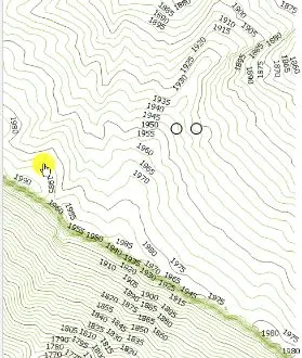
Next, create contours, a vector file, from your ground raster (DEM), using the create contours tool. Change the basemap to imagery to visualize the contours against a satellite image. To create index contours, use the Contour with Barriers tool. To do this, do not actually indicate a “barriers” layer but rather use the contour with barrier tool to achieve an “index” contour, as I did, shown below. I used 5 for the contour interval and 25 (every fifth contour) for the index contour interval. This results in a polyline feature class with a field called “type”. This field receives the value of 2 for the index contours and 1 for all other contours. Now, simply symbolize the lines as unique value on the type field, specifying a thicker line for the index contours (type 2) and a thinner line for all the other contours.
Next, convert your 2D map to a 3D scene using the Catalog pane. If you wish, undock the 3D scene and drag it to the right side of your 2D map so that your 2D map and 3D scene are side by side. Use View > Link Views to synchronize the two. Experiment with changing the base map to topographic or terrain with labels. Or, if your area is in the USA like mine is, use the Add Data > USA topographic > add the USGS topographic maps as another layer. The topographic maps are at 1:24,000 scale in the most detailed view, and then 1:100,000 and 1:250,000 for smaller scales.
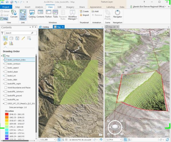
2D and 3D synced views of the contours symbolized with the Contours with Barriers tool in ArcGIS Pro.
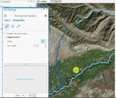
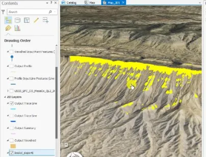
At this point, the sky’s the limit for you to conduct any other type of raster-based analysis, or combine it with vector analysis. For example, you could run the profile tool to generate a profile graph of a drawn line (as I did, shown below) or an imported shapefile or line feature class, create a viewshed from your specified point(s), trace downstream from specific points, determine which areas in your study site have slopes over a certain degree, or use the Lidar and derived products in conjunction with vector layers to determine the optimal site for a wildfire observation tower or cache for firefighters.


Profile graph of the cyan polyline that I created from the Lidar data from the National Map in ArcGIS Pro.
Tracing downstream using the rasters derived from the lidar data in ArcGIS Pro.
Slopes over 40 degrees using the slope raster derived from the lidar data in ArcGIS Pro.
I hope these procedures will be helpful to you.
You must be a registered user to add a comment. If you've already registered, sign in. Otherwise, register and sign in.
-
Administration
89 -
Announcements
85 -
Career & Tech Ed
1 -
Curriculum-Learning Resources
280 -
Education Facilities
24 -
Events
77 -
GeoInquiries
1 -
Higher Education
616 -
Informal Education
284 -
Licensing Best Practices
102 -
National Geographic MapMaker
39 -
Pedagogy and Education Theory
239 -
Schools (K - 12)
282 -
Schools (K-12)
302 -
Spatial data
39 -
STEM
3 -
Students - Higher Education
257 -
Students - K-12 Schools
142 -
Success Stories
44 -
TeacherDesk
1 -
Tech Tips
125
- « Previous
- Next »