- Home
- :
- All Communities
- :
- Products
- :
- ArcGIS Spatial Analyst
- :
- ArcGIS Spatial Analyst Blog
- :
- Doing more with Euclidean Distance: Barriers and P...
Doing more with Euclidean Distance: Barriers and Paths
- Subscribe to RSS Feed
- Mark as New
- Mark as Read
- Bookmark
- Subscribe
- Printer Friendly Page
- Report Inappropriate Content
Currently, Euclidean Distance Mapping geoprocessing tools can be used to assign distance properties to raster cells. Example applications include distance from runways used as part of an airport noise model, or distance from streams used as a criterion layer in a habitat suitability model. From ArcGIS Pro 2.4 and ArcMap 10.7.1, you can now use the Euclidean distance tool to consider an important use case: generating precise shortest paths around barriers. You can also use barrier-aware distance and allocation maps to replace their corresponding cost distance versions as input layers in suitability models.
Consider these related use cases posted to geonet:
- “Aim: To determine the shortest path from a nest to marine foraging locations for an individual bird. The bird is restricted to traveling along water only (i.e., freshwater and ocean).” [1]
- “I have been running some least cost path analyses on manatee GPS telemetry data using ArcGIS 9.3.1. The goal of this analysis is to create the shortest path between points without the path crossing land.” [2]
Prior to ArcGIS Pro 2.4/ArcMap 10.7.1, the only way to plot shortest paths around barriers was to use the Cost Distance (CD) tool using a constant cost surface with a small, positive, non-zero cost for the areas where movement was allowed and either a high cost or nodata where movement was prohibited. As the geonet posters point out, the cost paths obtained from this approach are unsatisfactory. To drive this point home, lets recreate the seabird flight paths (using completely fake nesting and feeding site data) using the CD + constant cost surface approach. The study area is Vancouver, British Columbia.
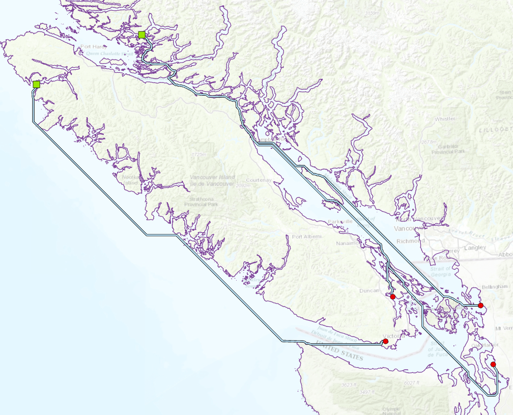
Figure 1: Sea bird over-water flight paths created using the CostDistance + constant cost surface approach. The Cost Distance sources are the feeding sites in the northwest corner and the Cost Path As Polyline destinations are the nesting locations in the southeast corner.
Goodchild [3] discusses why these paths deviate. The underlying cost distance algorithm is based on an 8-way connected graph, which restricts the directions that can be considered, and the absence of meaningful variation in the cost surface (other than barriers) means that the CostPath/CostPath As Polyline operation doesn’t know which of many equal length routes to choose from.
At 2.4/10.7.1, we can do better, as shown below in figure 2 in green, using enhancements to the Euclidean Distance (ED) and Cost Path As Polyline GP tools.

Figure 2: Sea bird over-water flight paths (in green) created using barrier-aware Euclidean Distance and Cost Path As Polyline tools.
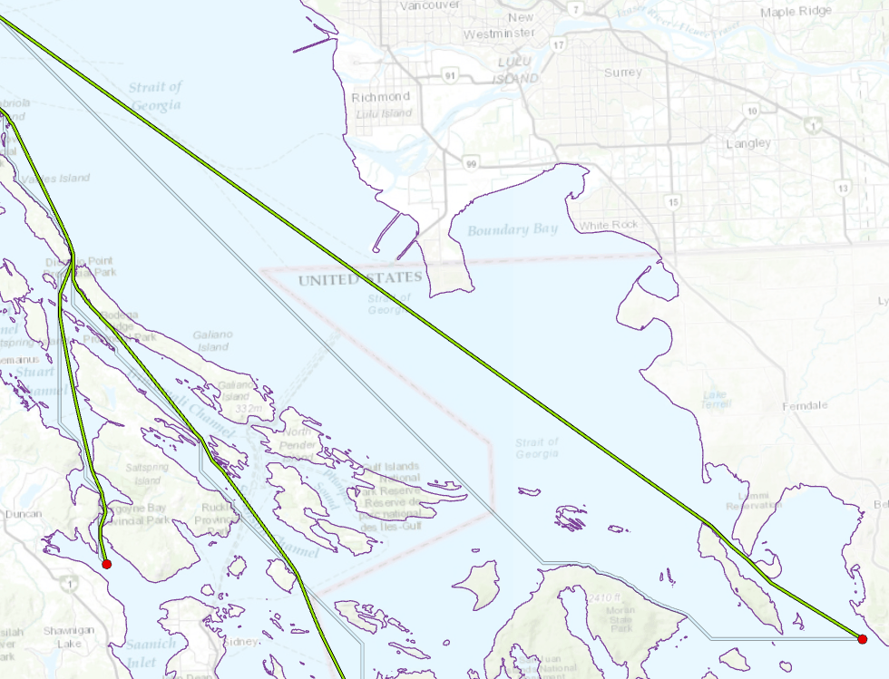
Figure 3: Detail showing Euclidean distance (in green) and Cost Distance (in blue) flight paths.
The CD paths in this example are only about 1% longer than the ED paths, but their deviations from the geometric shortest paths are significant.
There is also a geodesic option for ED, but we haven’t used it in this example because we wanted to compare results with CD.
Creating Shortest Paths With Barriers
To generate these improved paths, use the following workflow:
1. Create a barrier dataset. It can be any kind of feature class or a raster. In the example above, the barrier dataset is a polyline feature class representing coastlines. If it’s a raster, DATA cells act as barriers.
2. Use the Euclidean Distance tool instead of the Cost Distance tool. Specify values for the new optional input parameter “Input raster or feature barrier data” and the new optional output parameter “Out back direction raster”, as shown below:
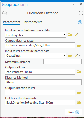
Figure 4: Euclidean distance tool user interface
3. Use the Cost Path As Polyline tool to create the paths from the destinations (Nesting sites) back to the sources (Feeding Sites). This tool has been enhanced to accept the new back direction output from Euclidean distance:
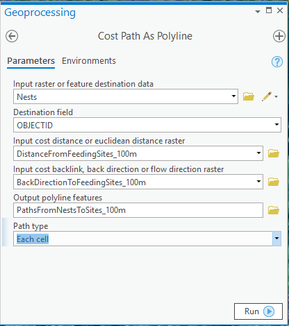
Figure 5: Cost Path As Polyline tool user interface
Simple!
The Back Direction Raster
The new back direction raster, created by the Euclidean toolset, encodes a floating point azimuth value in the range (0.0, 360.0] degrees, with zero itself reserved for source cell locations. This azimuth points in the direction of the shortest path as it passes through the cell. This is different than the “Output direction raster” parameter, which uses the 1-360 azimuth value (rounded to an integer) to point directly at the closest source cell (the cell where the shortest path will eventually end).
You can always ask for the back direction raster to be generated whether or not barriers are specified. This provides a convenient way to use Cost Path As Polyline tool to identify which source cell is closest to a given destination cell (it’s the cell on which the polyline ends) even if you’re not interested in barriers or specific pathways. Locating this cell was difficult in earlier versions of the Euclidean toolset: For planar Euclidean distance, you could have done some math with the distance and direction outputs, but that wouldn’t work for geodesic output.
Barrier-aware Distance and Allocation Outputs
So far, we’ve emphasized the use of the new functionality in generating better shortest paths. For this application, the most important output was the new back direction raster, which gave Cost Path as Polyline the information it needed to plot those paths step-by-step.
The distance and allocation maps may also be directly useful. As an example, compare the euclidean and cost distance versions of the barrier-aware distance map in figures 6 and 7 below. The euclidean version avoids the distortions present in the cost distance version.
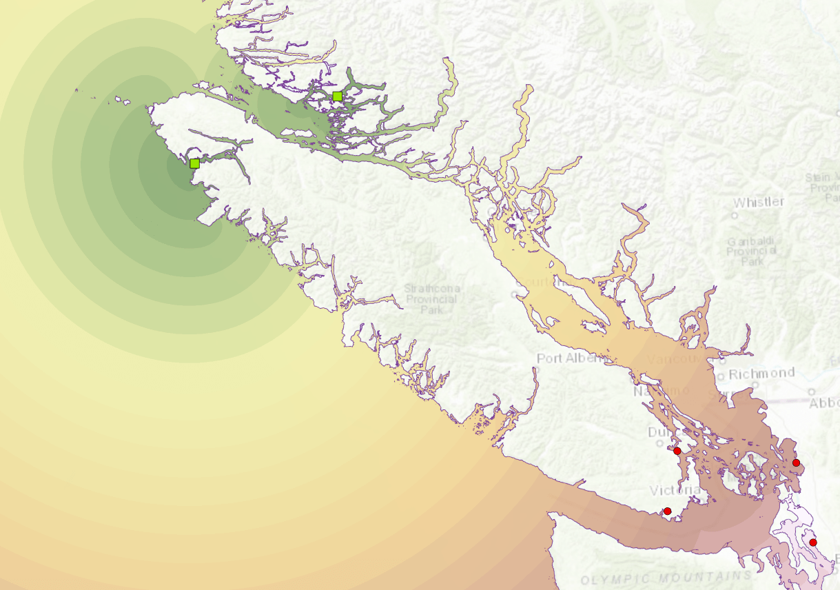
Figure 6: Barrier-aware Euclidean distance map used to compute the sea bird over-water flight paths.
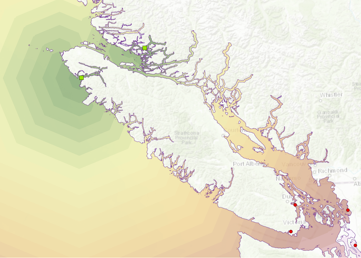
Figure 7: Cost distance map produced from encoding coastline as nodata into a constant cost surface
Use of Distance and Allocation Outputs in Suitability Models
Let’s repeat that the difference between CostDistance and Euclidean Distance with barriers is that the former performs its computation using a network distance metric and the latter uses a euclidean distance metric. This is something to be aware of when using the outputs of cost distance as layers in a suitability model. It is probably the case that some other layers in that model assume a Euclidean distance metric, so the mixture of distance metrics in a single suitability model will introduce some amount of error into the model results. For example, if both the Cost allocation and Euclidean allocation datasets shown in the figure below were used in the same model, then the classification of cells near an allocation boundary becomes more uncertain, as shown below.
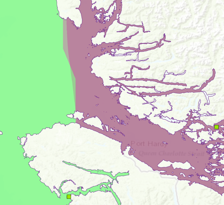
Figure 8: Comparison between cost allocation and barrier-aware euclidean allocation zones. Note the zig-zag distortion in the cost allocation boundary.
The only reason to mix distance metrics like this is because, up until now, there hasn’t been a good alternative. Also, the distance distortion itself is bounded by a factor of about 1.1 ([3, Table 2], so that may be good enough for many applications. However, now we have a better alternative for the special case of barriers on a constant cost surface. For a distortion free solution for more general cost distance problems, we’ll have to wait for an upcoming ArcGIS platform release.
Summary
This blog has shown you how to generate shortest paths around barriers, using the versions of the Euclidean Distance and Cost Path as Polyline tools available in ArcGIS Pro 2.4 and ArcMap 10.7.1. Also, if you are using cost distance tools with a constant cost raster (containing some nodata cells) to generate inputs for a suitability model, you should consider using the barrier-aware euclidean tools instead.
References
[1] Sea bird geonet posting
https://community.esri.com/thread/109625
[2] ManateeGISDB geonet posting
https://community.esri.com/thread/97784-least-cost-path-anomalies
[3] Description of length and direction distortions in current cost distance implementation
Goodchild, M. F. (1977). An Evaluation of Lattice Solutions to the Problem of Corridor Location. Environment and Planning A. 9. 727-738. 10.1068/a090727.
[4] Readable introduction to barrier-aware euclidean distance method
Sethian, J. A. (1997). Tracking Interfaces with Level Sets: An “act of violence” helps solve evolving interface problems in geometry, fluid mechanics, robotic navigation and materials sciences. American Scientist Vol. 85, No. 3 (MAY-JUNE 1997), pp. 254-263
The original blog is available at https://www.esri.com/arcgis-blog/products/spatial-analyst/analytics/doing-more-with-euclidean-distan...
The content of the blog has been prepared by James TenBrink, a senior software engineer in the raster analysis group at esri. He has a Bachelor of Science degree in Computer Science from Hope College in Holland, Michigan, and a Master of Science degree in Computer Science from Rensselaer Polytechnic Institute in Troy, New York. He has been with Esri 28 years and has had an office in almost every building, on almost every floor, of the Esri campus.
You must be a registered user to add a comment. If you've already registered, sign in. Otherwise, register and sign in.