ArcGIS GeoStatistical Analyst Blog

cancel
Showing results for 
Show  only  | Search instead for 
Did you mean: 

Latest Activity

(5 Posts)
EricKrause
Esri Regular Contributor

We are happy to announce that Empirical Bayesian Kriging (EBK) has been fully peer-reviewed, and the methodology has been accepted into August edition of the Spatial Statistics journal.

https://www.sciencedirect.com/science/article/pii/S2211675319300168

This is the reference you should cite if you need to academically cite Empirical Bayesian Kriging, EBK Regression Prediction, or Empirical Bayesian Kriging 3D in your work or studies.  

The article contains an overview of the methodology behind EBK, as well as many results from controlled simulations.  The results are very impressive, and they show that EBK performs as well (and often better) than other modern interpolation routines in a variety of situations.  It also contains recommendations for when the default parameters are sufficient and when more advanced parameters should be considered.

more
0 0 600
EricKrause
Esri Regular Contributor

In the newly released ArcGIS Pro 2.3 (available through MyEsri),  Geostatistical Analyst has made available the first 3D interpolation method in ArcGIS, Empirical Bayesian Kriging 3D.  This method takes points with x, y, and z coordinates and a measured value and interpolates the measured value into a continuous 3D model using Empirical Bayesian Kriging methodology.

Geostatistical layer in 3D

The result of the interpolation is visualized as a horizontal slice at a particular elevation, and the current elevation can be changed with the Range slider.  The animation above shows the Range slider moving through thirty different elevations.

Watch of video of Empirical Bayesian Kriging 3D

Read more about Empirical Bayesian Kriging 3D

Interpolate 3D Oxygen Measurements in Monterey Bay has been created as a LearnGIS lesson.  This lesson teaches how to perform 3D interpolation using dissolved oxygen measurements in Monterey Bay.  You will learn how to explore the oxygen measurements, perform EBK3D as a geoprocessing tool and in the Geostatistical Wizard, assess the accuracy using cross validation, and export the interpolation results to contours, rasters, and 3D animations. 

more
2 19 5,115
EricKrause
Esri Regular Contributor

It's almost time for the 2018 Esri User Conference (July 9-13). We here on the Geostatistical Analyst team are busy practicing and polishing our presentations, and we are looking forward to showing you what we’ve been working on since last summer.  If you do any kind of sample data prediction for spatial data analysis and decision making, please look at the guide below to help you plan out your time with us.


See the full agenda for more details on these sessions, and more. Be sure to download the Esri Events Mobile App too!

Please come by the Island in the Showcase during the week (Tuesday and Wednesday from 9 – 6, and Thursday from 9 – 1:30).  We’d love to hear about the work you do, any difficulties you encounter, and any ideas you might have to make our software suit your needs even better.

Finally, remember to check out the Spatial Analysis: The Road Ahead session for a peek into the future.

more
0 0 512
EricKrause
Esri Regular Contributor

A new subsetting algorithm has been developed in Geostatistical Analyst for ArcGIS Pro 2.1, Generate Subset Polygons, as a geoprocessing tool. The purpose of this tool is to break down the spatial data into small, nonoverlapping subsets.

The new tool is intended to be used to create Subset Polygons in EBK Regression Prediction and any future tools that allow you to define subsets using polygons.

Why do we need a new subsetting algorithm?

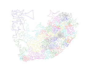
The current subsetting algorithm implemented in Empirical Bayesian Kriging (EBK) and EBK Regression Prediction often encounters problems with clustered data. For example, in the figure below, the current subsetting algorithm often combines data far away from each other into the same subset. This is not desirable because the subsets should be as compact as possible.

Figure 1: Overlapping subsetting polygon using EBK Regression Prediction, where the blue dots are the point location of rainfall stations and the selected polygon (cyan) shows the overlapping nature. The data for this analysis have been taken from [1].

Figure 1: Overlapping subsetting polygon using EBK Regression Prediction, where the blue dots are the point location of rainfall stations and the selected polygon (cyan) shows the overlapping nature. The data for this analysis have been taken from [1].

The new algorithm

In the new algorithm, for each subset Si, the number of points ni satisfies the constraint min ≤ ni ≤max and minimizes the sum of the pairwise squared deviations within the subsets ∑i ∑xSi ∑ySi ||x-y||2. This could also be reorganized as the sum of weighted variances within the subsets 2∑nxSi ||x- ci||2, where ci is the center of the subset Si. Note, this algorithm has a harsher penalty on the number of points in each subset as compared to the K-mean clustering.

The new algorithm performs the following three steps:

Step 1: Connects all points and form a closed curve.

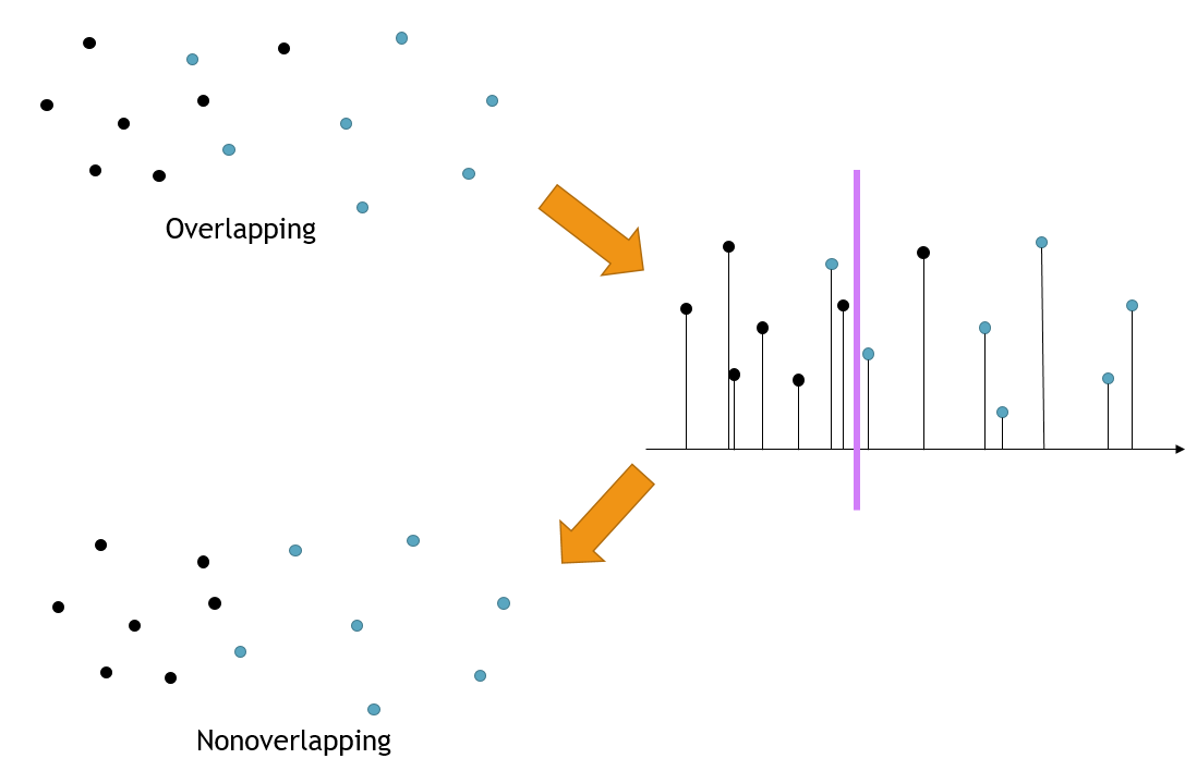
Step 2: Cuts the curve into subsets.

Step 3: Finds all overlaps and resolves them.

Step 1

The first step connects all points and forms a closed curve. To achieve this, we form a grid in the work space and put all points that are regarded as clusters into corresponding grid cells.

Figure 2: Example of how the points are connected to form a closed curve.

If two clusters are in the same cell, we merge them into one. A hash table is used to locate the clusters in the grid for efficient searching. We merge nearby clusters to form the curve. Initially, the cell size is extremely fine to ensure that points are connected locally. As the size of the cluster increases, the cell size also increases. The time complexity of this step is O(n · log n), where n is the total number of points.

Step 2

The second step cuts the curve into subsets. While cutting the curve, we satisfy the constraint on the number of points in each subset and minimize the sum of the pairwise squared deviations within the subsets. A dynamic programming algorithm is applied to solve this task. The complexity of the algorithm is O((max-min) · n).

Figure 3: The curve is cut into subsets, where the number of points in each subset satisfies the minimum and maximum requirement, and the sum of the pairwise squared deviations within the subsets are minimized.

Step 3

The third step finds all overlaps and resolves them while further minimizing the sum of the pairwise squared deviations within the subsets. At present, we are using a brute force search in the third step, which accounts for most of the total execution time (with complexity O(n2)), to find overlapping subset pairs. The overlapping is resolved by finding a partitioning between the two subsets, minimizing the sum of the pairwise squared deviations within each subset, while maintaining the required minimum and maximum number of points in each subset. This is performed by projecting points to a set of directions in n-dimension covering the space evenly. For each projection, the optimal division can be found by a dynamic programming approach. Among all projections, the one with the minimum penalty is chosen. The algorithm iterates until no overlaps are detected or the number of iterations reaches the upper bound. The figure below shows a single overlap being removed.

Figure 5: Finding and resolving overlaps within the subsets.

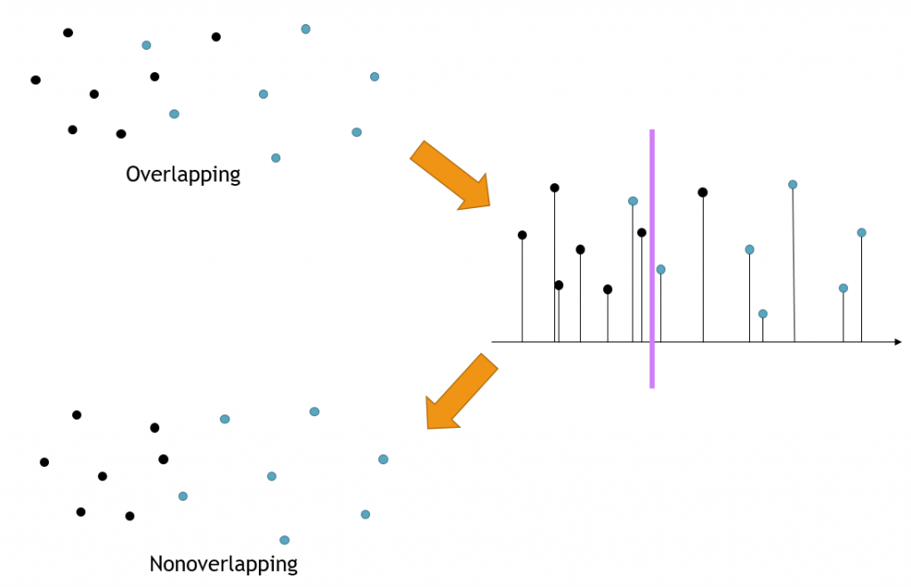
Figure 4: Finding and resolving overlaps within the subsets.

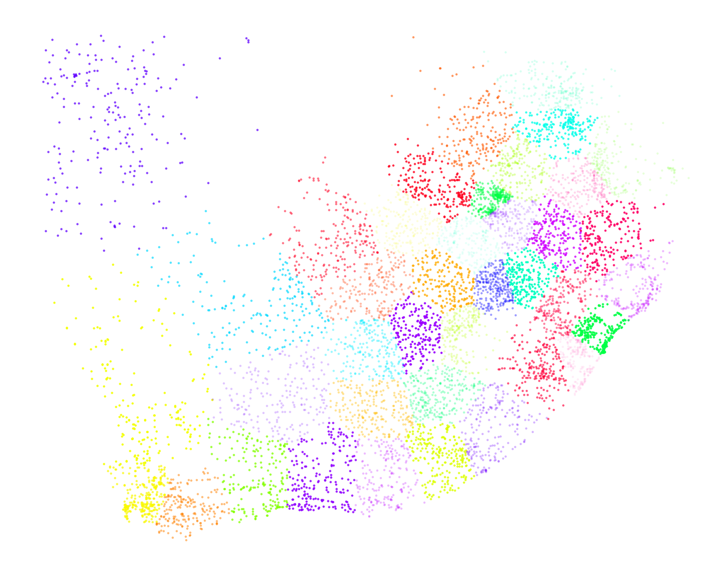
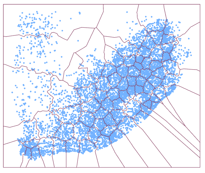
The new subsetting algorithm classifies each point into a subset (Figure 5) and creates polygons that wrap around each individual subset (Figure 6).  Thus, for each polygon, all points inside the polygon belong to the same subset.

Figure 6: The new subsetting algorithm produces non-overlapping subset.

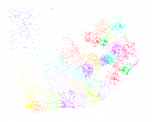
Figure 5: Non-overlapping subsets.

Figure 7: The non-overlapping subsets produces the final tool output which are represented by non-overlapping polygons.

Figure 6: The non-overlapping subsets produces the final tool output which are represented by non-overlapping polygons.

Performance analysis of the new algorithm

Overall, the time complexity of the whole algorithm is O(n2), given the high computational complexity of searching for overlapped subsets.

The figure below shows the time complexity of the three steps as well as each function plotted on the same graph.  In the current implementation, the third step takes the vast majority of the computation time for large numbers of points.

Figure 8: Time complexity of the algorithm in the three stages.

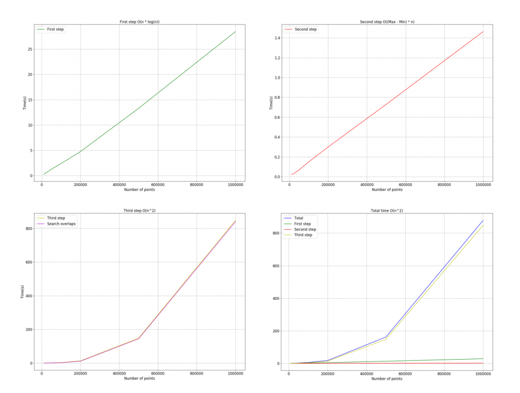
Figure 7: Time complexity of the algorithm in the three stages.

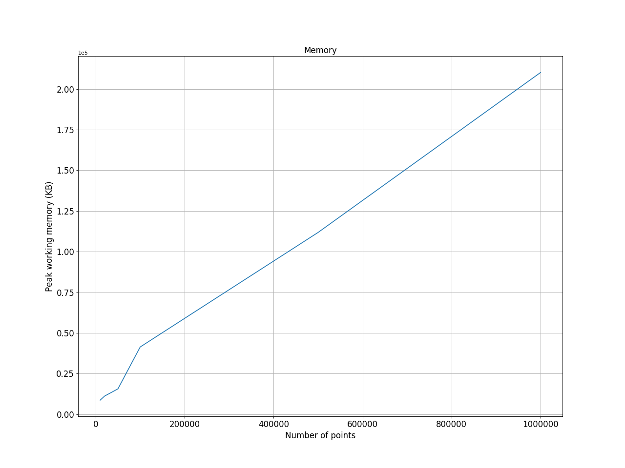
The space complexity of the algorithm is O(n), which means that the required memory is proportional to the number of points. The following image shows the memory allocation is linear with the number of input points.

Figure 9: Space complexity of the algorithm.

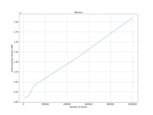
Figure 8: Space complexity of the algorithm.

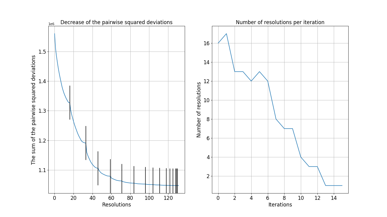
The following graphs show the analysis of the algorithm in the third step (resolution of overlapping subsets). When two subsets overlap, resolving their overlap reduces the total sum of the pairwise squared deviations. The graph on the left shows the decrease in the total sum after each resolution. The graphs on the right shows the number of resolutions in each iteration. For this data, the algorithm converges after about 14 iterations.

Figure 10: Analysis of the algorithm in the third step where overlapping subsets are resolved.

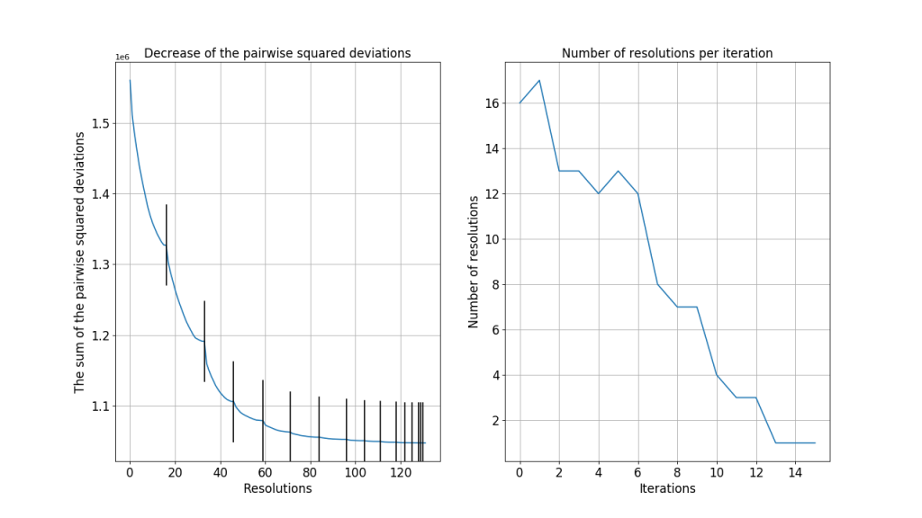
Figure 9: Analysis of the algorithm in the third step where overlapping subsets are resolved.

Application

This new subsetting algorithm can work efficiently with clustered datasets with more than a billion points. The quality of the constructed subsets in the new subsetting algorithm is often better than the algorithm currently used in EBK. Though it does not yet support 3D points, the methodology can be easily extended to multiple dimensions.

Part of this new subsetting algorithm and blog content was created by Zeren Shui, advised by Alexander Gribov, during his internship with the Geostatistical Analyst Team in summer 2017. Zeren is currently pursuing his Master’s degree in Data Science at College of Science and Engineering, University of Minnesota – Twin Cities. His research interests are Bayesian Statistics, Machine Learning, and Data Mining. For additional questions, you can comment here or contact him at shuix007@umn.edu.

References

[1] S. D. Lynch, Development of a raster database of annual, monthly and daily rainfall for southern Africa, WRC Report (1156/1/04) (2004) 78.

more
1 0 639
EricKrause
Esri Regular Contributor

Spatial interpolation is one of the most common workflows in GIS, and the Geostatistical Analyst extension is built specifically to solve this problem. However, there is often confusion about how exactly interpolation should be done.  Which interpolation method should I use?  Which parameters should I use?  How do I know if the interpolated surface can be trusted?  These questions frequently seem daunting to people when they first approach spatial interpolation, and the purpose of this blog is to help you get started towards your goal of accurate spatial interpolation.


Don’t have Geostatistical Analyst?  Try Geostatistical Analyst for free.


As a starting point, we suggest the Geostatistical Analyst tutorial:

  1. Download the ArcGIS Tutorial Data for Desktop through my.esri.com.  You must have an up-to-date license for ArcGIS for Desktop to download the tutorial data.
  2. There are five tutorials that you should complete.  It will take a few hours to finish all of them:
    1. Introduction to the ArcGIS Geostatistical Analyst Tutorial
    2. Exercise 1: Creating a surface using default parameters
    3. Exercise 2: Exploring your data
    4. Exercise 3: Mapping ozone concentration
    5. Exercise 4: Comparing models
    6. Exercise 5: Mapping the probability of ozone exceeding a critical threshold


Once you have seen the videos and done the tutorial exercises, you should be ready to start using Geostatistical Analyst on your own data.  If you need additional education material, the following Web Courses are available:


If you have reviewed the training material above but still have questions, feel free to post your questions to GeoNet at the Geostatistical Analyst Place.


Good luck and happy kriging!


------------------------------------------------------------------------------------


Geostatistical Analyst also has extensive documentation that is available for free online.  Here are a few select topics about some of the most important features in the extension:


------------------------------------------------------------------------------------

UPDATE (September 2017) - Free textbook and data


I am happy to announce that we have made Spatial Statistical Data Analysis for GIS Users available as a free download. 


This textbook, written by Konstantin Krivoruchko, was previously available through Esri Press:  "This book presents a practical introduction and guide to spatial statistics for researchers, statisticians, academics, and college students who want to expand their knowledge and skills in geographic information system (GIS) technology to new areas of analysis. More than 1,000 full-color illustrations are included, along with lessons and sample data to help organize courses and lectures."


Download link for the PDF book: https://downloads.esri.com/esripress/pdfs/spatial-statistical-data-analysis-for-gis-users.pdf

Download link for datasets used in the book: https://downloads.esri.com/esripress/pdfs/spatial-statistical-data-analysis-for-gis-users.zip


------------------------------------------------------------------------------------

UPDATE (May 2018, February 2019) - LearnGIS exercises using Geostatistical Analyst


Several LearnGIS exercises have been created that make heavy use of Geostatistical Analyst.  LearnGIS lessons are free online exercises that teach different concepts related to geographic analysis in real-world workflows.  They are a great way to see geostatistical workflows from beginning to end.


-------------------------------------------------------------------------------------

UPDATE (July 2019) - "Evaluation of empirical Bayesian kriging" has been peer-reviewed and published in the August issue of the Journal of Spatial Statistics.  This paper presents the theory and principles behind EBK as well as results from controlled simulations.  The results show EBK is accurate and valid for a wide variety of data and generally performs very well compared to other modern interpolation methods.

https://www.sciencedirect.com/science/article/pii/S2211675319300168


-------------------------------------------------------------------------------------

UPDATE (June 2020) - "Empirical Bayesian kriging implementation and usage" has been published in the June 2020 edition of "Science of The Total Environment."  This peer-reviewed paper contains the details of the mathematical underpinnings of Empirical Bayesian kriging.

https://www.sciencedirect.com/science/article/pii/S0048969720308007 

more
8 0 5,708
59 Subscribers