Turn on suggestions
Auto-suggest helps you quickly narrow down your search results by suggesting possible matches as you type.
Cancel
- Home
- :
- All Communities
- :
- Services
- :
- Esri Technical Support
- :
- Esri Technical Support Blog
- :
- Classifying Images in ArcGIS for Desktop 10.4
Classifying Images in ArcGIS for Desktop 10.4
Subscribe
6074
0
07-13-2016 11:58 AM
- Subscribe to RSS Feed
- Mark as New
- Mark as Read
- Bookmark
- Subscribe
- Printer Friendly Page
- Report Inappropriate Content
07-13-2016
11:58 AM
With the addition of the Train Random Trees Classifier, Create Accuracy Assessment Points, Update Accuracy Assessment Points, and Compute Confusion Matrix tools in ArcMap 10.4, as well as all of the image classification tools in ArcGIS Pro 1.3, it is a great time to check out the image segmentation and classification tools in ArcGIS for Desktop. Here we discuss image segmentation, compare the four classifiers (Train Iso Cluster Classifier, Train Maximum Likelihood Classifier, random trees, and Support Vector Machine), and review the basic classification workflow.Image Segmentation
Before you begin image classification, you may want to consider segmenting the image first. Segmentation groups similar pixels together and assigns the average value to all of the grouped pixels. This can improve classification significantly and remove speckles from the image.Train Iso Cluster Classifier
The Iso Cluster is an unsupervised classifier (that is, it does not require a training sample), with which the user can set the number of classes and divide a multiband image into that number of classes. This classifier is the easiest of all the classifiers to use, as it does not require creating a training sample and can handle very large segmented images. However, this classifier is not as accurate as the other classifiers due to the lack of training sample.Train Maximum Likelihood Classifier
The Maximum Likelihood Classifier (MLC) uses Bayes' theorem of decision making and is a supervised classifier (that is, the classifier requires a training sample). The training data is used to create a class signature based on the variance and covariance. Additionally, the algorithm assumes a normal distribution of each class sample in the multidimensional space, where the number of dimensions equals the number of bands in the image. The classifier then compares each pixel to the multidimensional space for each class and assigns the pixel to the class that the pixel has the maximum likelihood of belonging to based on its location in the multidimensional space.Train Random Trees Classifier
One supervised classifier that was introduced with ArcGIS 10.4 is the random trees classifier, which breaks the training data into a random sub-selection and creates classification decision trees for each sub-selection. The decision trees run for each pixel, and the class that gets assigned to the pixel most often by the trees is selected as the final classification. This method is resistant to over-fitting due to small numbers of training data and/or large numbers of bands. This classifier also allows the inclusion of auxillary data, including segmented images and digital elevation model (DEM) data.Train Support Vector Machine Classifier
Support Vector Machine (SVM) is a supervised classifier similar to the MLC classifier, in that the classifier looks at multidimensional points defined by the band values of each training sample. However, instead of evaluating the maximum likelihood that a pixel belongs to a class cluster, the algorithm defines the multidimensional space in such a way that the gap between class clusters is as large as possible. This divides the space up into different sections separated by gaps. Each pixel is classified where it falls in the divided space.Image Classification Workflow:
With the addition of the Create Accuracy Assessment Points, Update Accuracy Assessment Points, and Compute Confusion Matrix tools in ArcGIS 10.4, it is now possible to both create and assess image classification in ArcMap and ArcGIS Pro.
The general workflow for image classification and assessment in ArcGIS is:
The best part about this six-step process is that it makes it pretty easy to compare different classification methods, and it’s often important to compare the different methods. Getting your training sites nailed down (step 2) is usually the toughest part, but steps 3 through 7 fly by since the analysis is done for you. In the end, you have several classified raster images to use in your work and can choose the best result based on your personal objectives.
As an example, we used this workflow to classify a Landsat 8 image of the Ventura area in Southern California. We used the MLC, SVM, and Random Trees (RT) methods to classify a single Landsat 8 raster captured on February 15, 2016. We classified the image into nine classes and manually selected training samples and accuracy assessment (“ground truth”) points. Additionally, we used a segmented image as an additional input raster for each classifier. Once we classified the rasters, we computed a confusion matrix for each output to determine the accuracy of the classification when compared to ground truth points. The Kappa index in the Confusion Matrix gives us an overall idea of how accurate each classification method is.
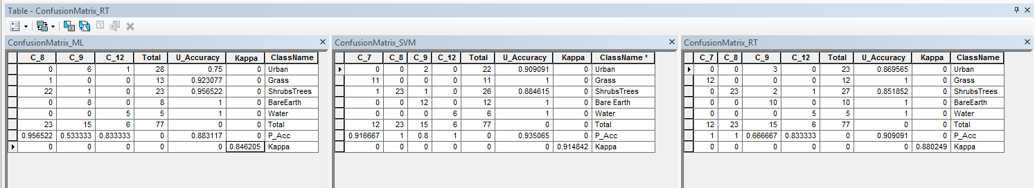
The results showed that each method did pretty well in the classification when looking at the Kappa indexes, as well as based on a visual assessment. In order of accuracy (from the highest Kappa index to the lowest), we see that the SVM output was the most accurate (Kappa = 0.915), followed by Random Trees (Kappa = 0.88) and finally the MLC method (Kappa = 0.846).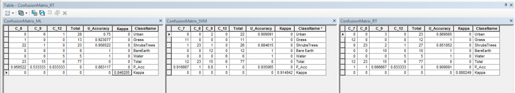
We can see from the Confusion Matrix that some methods did better than others for specific classes. For example, the MLC didn’t do too well with Bare Earth classification, but RT and SVM weren’t too much better. This is great information for honing in on a better-classified image–now we know that we should focus on getting better Bare Earth training samples to improve our results. You could keep going with this until you get a really high accuracy for all classes, if that’s what you need for your analysis. If you need just a general idea of the area, you could just take what you get in Round 1! Check out what we got:
Source image: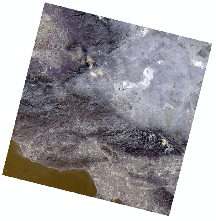
Classified Image: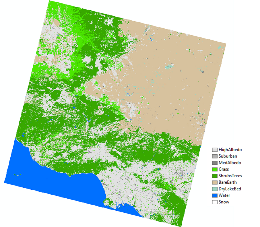
Make sure to check out the new Image Classification Wizard with the release of ArcGIS Pro 1.3!
Julia L. and Rebecca R. - Desktop Support
Before you begin image classification, you may want to consider segmenting the image first. Segmentation groups similar pixels together and assigns the average value to all of the grouped pixels. This can improve classification significantly and remove speckles from the image.Train Iso Cluster Classifier
The Iso Cluster is an unsupervised classifier (that is, it does not require a training sample), with which the user can set the number of classes and divide a multiband image into that number of classes. This classifier is the easiest of all the classifiers to use, as it does not require creating a training sample and can handle very large segmented images. However, this classifier is not as accurate as the other classifiers due to the lack of training sample.Train Maximum Likelihood Classifier
The Maximum Likelihood Classifier (MLC) uses Bayes' theorem of decision making and is a supervised classifier (that is, the classifier requires a training sample). The training data is used to create a class signature based on the variance and covariance. Additionally, the algorithm assumes a normal distribution of each class sample in the multidimensional space, where the number of dimensions equals the number of bands in the image. The classifier then compares each pixel to the multidimensional space for each class and assigns the pixel to the class that the pixel has the maximum likelihood of belonging to based on its location in the multidimensional space.Train Random Trees Classifier
One supervised classifier that was introduced with ArcGIS 10.4 is the random trees classifier, which breaks the training data into a random sub-selection and creates classification decision trees for each sub-selection. The decision trees run for each pixel, and the class that gets assigned to the pixel most often by the trees is selected as the final classification. This method is resistant to over-fitting due to small numbers of training data and/or large numbers of bands. This classifier also allows the inclusion of auxillary data, including segmented images and digital elevation model (DEM) data.Train Support Vector Machine Classifier
Support Vector Machine (SVM) is a supervised classifier similar to the MLC classifier, in that the classifier looks at multidimensional points defined by the band values of each training sample. However, instead of evaluating the maximum likelihood that a pixel belongs to a class cluster, the algorithm defines the multidimensional space in such a way that the gap between class clusters is as large as possible. This divides the space up into different sections separated by gaps. Each pixel is classified where it falls in the divided space.Image Classification Workflow:
With the addition of the Create Accuracy Assessment Points, Update Accuracy Assessment Points, and Compute Confusion Matrix tools in ArcGIS 10.4, it is now possible to both create and assess image classification in ArcMap and ArcGIS Pro.
The general workflow for image classification and assessment in ArcGIS is:
- If desired, use the Segment Mean Shift tool to segment your imagery.
- Create a training sample using the Image Classification toolbar (if you are using the Iso Cluster classification, you can skip this step).
- Use one of the four training tools (Train ISO Cluster Classifier, Train Maximum Likelihood Classifier, Train Random Trees Classifier, Train Support Vector Machine Classifier).
- Use the Create Accuracy Assessment Points tool on the classified image to create randomly placed points that have values extracted from the image.
- Either use the Update Accuracy Assessment Point tool to compare this classification to previously created classifications, or manually edit the points and visually assess a reference image.
- Use the Compute Confusion Matrix tool to create a confusion matrix from the accuracy points.
- Use the measures of accuracy (the user’s accuracy, producer's accuracy, and Kappa index) calculated by the confusion matrix to assess the classification. Make changes to the training sample, as needed, to improve the classification.
The best part about this six-step process is that it makes it pretty easy to compare different classification methods, and it’s often important to compare the different methods. Getting your training sites nailed down (step 2) is usually the toughest part, but steps 3 through 7 fly by since the analysis is done for you. In the end, you have several classified raster images to use in your work and can choose the best result based on your personal objectives.
As an example, we used this workflow to classify a Landsat 8 image of the Ventura area in Southern California. We used the MLC, SVM, and Random Trees (RT) methods to classify a single Landsat 8 raster captured on February 15, 2016. We classified the image into nine classes and manually selected training samples and accuracy assessment (“ground truth”) points. Additionally, we used a segmented image as an additional input raster for each classifier. Once we classified the rasters, we computed a confusion matrix for each output to determine the accuracy of the classification when compared to ground truth points. The Kappa index in the Confusion Matrix gives us an overall idea of how accurate each classification method is.
The results showed that each method did pretty well in the classification when looking at the Kappa indexes, as well as based on a visual assessment. In order of accuracy (from the highest Kappa index to the lowest), we see that the SVM output was the most accurate (Kappa = 0.915), followed by Random Trees (Kappa = 0.88) and finally the MLC method (Kappa = 0.846).

We can see from the Confusion Matrix that some methods did better than others for specific classes. For example, the MLC didn’t do too well with Bare Earth classification, but RT and SVM weren’t too much better. This is great information for honing in on a better-classified image–now we know that we should focus on getting better Bare Earth training samples to improve our results. You could keep going with this until you get a really high accuracy for all classes, if that’s what you need for your analysis. If you need just a general idea of the area, you could just take what you get in Round 1! Check out what we got:
Source image:

Classified Image:

Make sure to check out the new Image Classification Wizard with the release of ArcGIS Pro 1.3!
Julia L. and Rebecca R. - Desktop Support
Labels
You must be a registered user to add a comment. If you've already registered, sign in. Otherwise, register and sign in.
Labels
-
Announcements
70 -
ArcGIS Desktop
87 -
ArcGIS Enterprise
43 -
ArcGIS Mobile
7 -
ArcGIS Online
22 -
ArcGIS Pro
14 -
ArcPad
4 -
ArcSDE
16 -
CityEngine
9 -
Geodatabase
25 -
High Priority
9 -
Location Analytics
4 -
People
3 -
Raster
17 -
SDK
29 -
Support
3 -
Support.Esri.com
60
- « Previous
- Next »