- Home
- :
- All Communities
- :
- Products
- :
- ArcGIS Data Interoperability
- :
- ArcGIS Data Interoperability Blog
- :
- ETL & File Geodatabase Views
ETL & File Geodatabase Views
- Subscribe to RSS Feed
- Mark as New
- Mark as Read
- Bookmark
- Subscribe
- Printer Friendly Page
- Report Inappropriate Content
This post shows some advanced ETL techniques but additionally shows how you can hand off finalizing your data to a geodatabase view (actually hundreds of them in this sample), letting the database do the heavy lifting, and in a File GDB at that. That's right - File Geodatabase views are a new feature at ArcGIS Pro 2.6, due out mid 2020, this is your preview! No longer are you confined to the 'where' clause in leveraging SQL when working with FileGDB!
I'm going big with the data behind the post - the USDA National Agricultural Statistics Service (NASS) crops database. I was thinking of calling the post something like 'You, Big Data and Asparagus' but that would lose a lot of people right at the title, even if they do like big data or asparagus. NASS is a big program, and I don't pretend to know all it offers, but for my demonstration purposes I'll use crop statistics per county. If you surf the NASS site you'll find ways to access data including selecting areas of interest using a map interface or as compressed text for data focusing on specific topics. I want it all, in bulk. NASS supports my need at this FTP site. The file names change daily, but look for the file beginning 'qs.crops'. At time of writing it contains over 19 million statistics for over 180 crop types, with records dating from the early 20th century. So, while the record count might not impress you, I'm going to call NASS 'Big Data' as it has a daily update velocity.
We're going to automate putting this data into File Geodatabase so it can be mapped and analyzed, and doing so at any frequency including the data's native daily lifecycle.
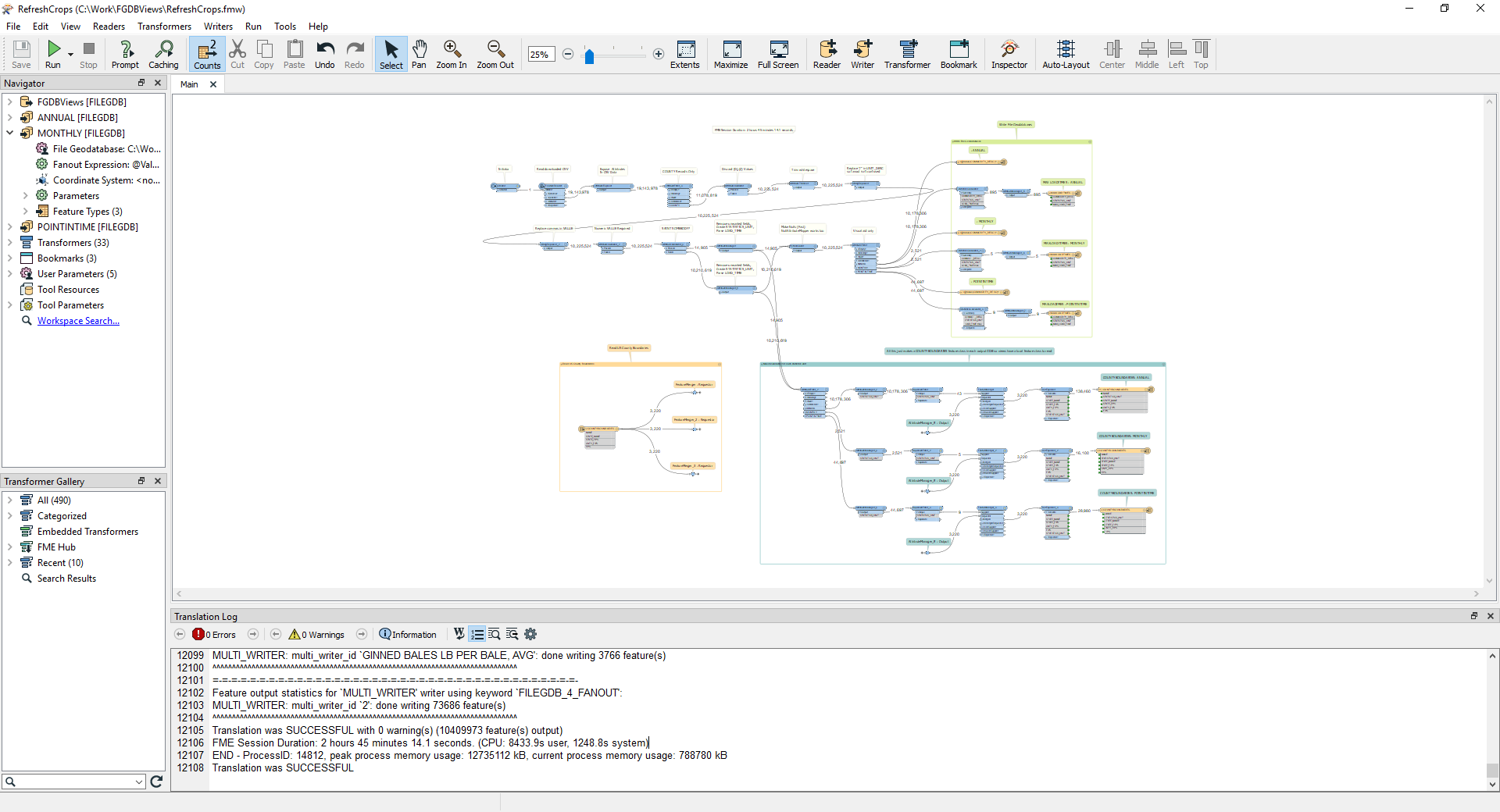
Importing the data to File GDB is done by the ETL tool RefreshCrops (in the post download). Here is how it looks after a successful run (click to enlarge), we'll walk through the underlying processing next. (I'm anticipating the reader is able to open the ETL tool, has some Workbench app experience, and will follow along; this requires Data Interoperability extension, or FME, both at release 2020 or later.)
The first issue with the data is that the file of interest changes name daily, so while you could read it with an FTPCaller transformer it would be an error-prone user experience to enter the correct URL for each run, so the process is automated with a Python scripted parameter. If you have never heard of scripted parameters before, they are a way to make user parameters work dynamically. We're breaking the no-code paradigm here, but we have a good reason. Here is how the parameter looks in the property editor:
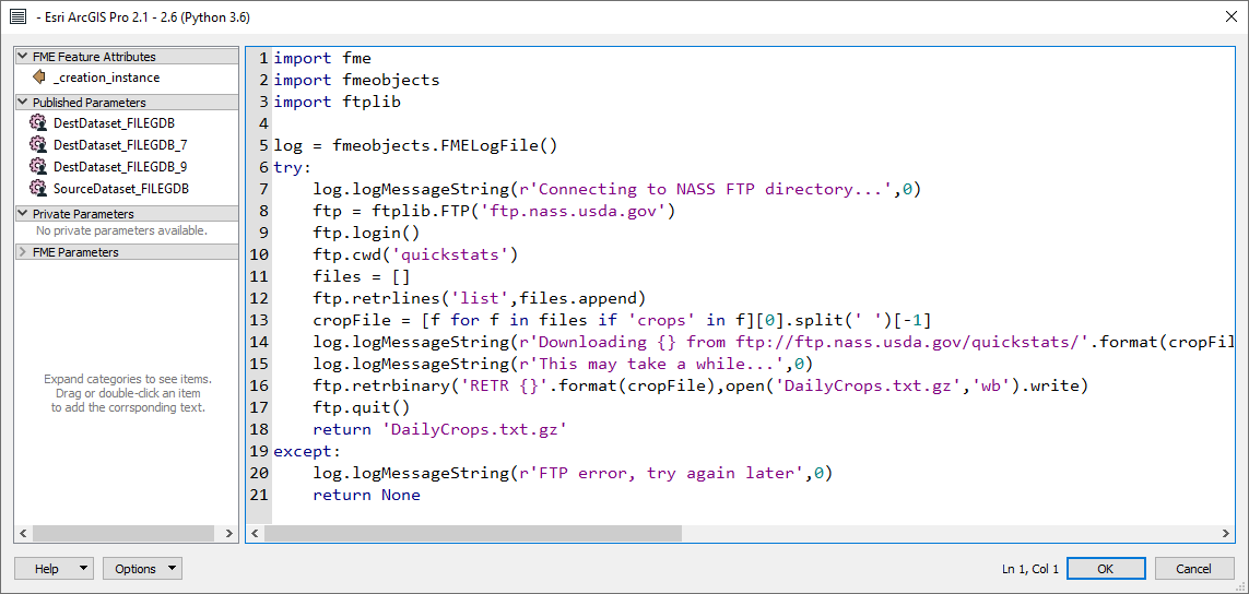
The code opens the FTP site, reads the available file names, then downloads the 'qs.crops' file to a file named DailyCrops.txt.gz. The file is written into the same folder as the ETL tool, namely the project home folder. On my laptop it takes a minute or two, and this occurs at the beginning of the tool run.
Now the GZipped payload has to be unpacked. It is delimited text data so can be opened with a FeatureReader using CSV format. CSV data rarely travels with a schema.ini file revealing its field types, but the schema is discoverable here, just click the Usage option. The file is however monolithic, containing all statistics for all crops and multiple aggregation areas (county, state, national) in just the one file, plus three aggregation periods (annual, monthly and point-in-time). For my purposes I'm interested only in statistics for the County level. So how do we separate the data by crop and county-level statistic? The technique is called fanout, in this case two types of fanout are used, dataset fanout that directs records into separate File GDBs for each statistic, and featuretype fanout that directs records into separate tables within each dataset.
The three output parameters (folders for annual, monthly and point in time statistics) have dataset fanout taken from the value of the STATISTICS_UNIT field, which is calculated at run time by concatenating STATISTICCAT_DESC and UNIT_DESC fields.
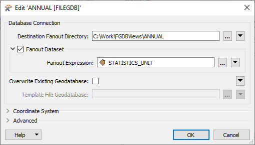
Each output dataset has writers for crop statistics where featuretype fanout is taken from the value of the COMMODITY_DESC field. Here is the property dialog for ANNUAL statistics:
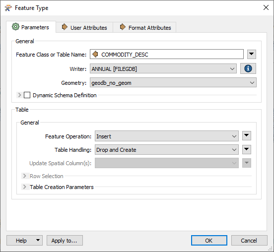
Note also the table handling property is set to Drop and Create, this is so re-runs of the tool remake each crop statistic table and don't keep adding to previously created data.
This combination of fanout settings dynamically creates 43 File GDBs for annual statistics, each with as many tables as there are crops reporting the statistic. There are smaller numbers of monthly and point-in-time workspaces output. Here is how the ANNUAL folder looks after the initial run (this takes a little less than 3 hours on my laptop):
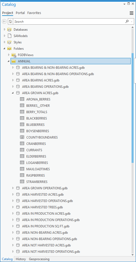
You can inspect the processing in the transformers that are outside of bookmarks and see that the basic idea is to ensure the VALUE field contains a valid numeric value and that the fanout attributes and state & county naming fields are well formed. The LOAD_TIME field is also made into a correct datetime value. Otherwise what went in is what comes out into each crop statistic table. Here is the schema:
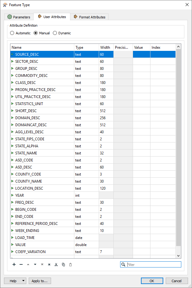
You will notice a feature class COUNTYBOUNDARIES is also copied into each output workspace so that the forthcoming view creation step can use objects within a single File GDB. A fine point; I use the API-based FILEGDB writer to output COUNTYBOUNDARIES as it has the ability to create an index on county and state name fields; the indexes will be used by the join processor when views are calculated. These indexes would be created automatically by the underlying Create Database View geoprocessing tool but I like to roll up these background tasks into my ETL.
Another output for each dataset is a table MAXLOADTIMES that shows the time of the latest load time for each crop statistic. More on this later.
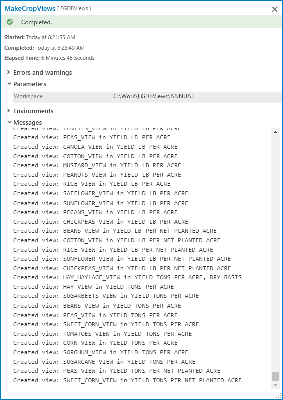
At this point we are ready for view creation. The input CSV data has no geometry, the whole point of the views is to join county boundary geometry to each crop statistic table. The script tool MakeCropViews walks each output dataset and creates views from all the crop statistic tables, using the Create Database View tool. For the ANNUAL folder this makes 895 views in a little over 15 minutes. Now that is a lot of data you don't have to generate manually!
Here is what you'll see in the message stream as MakeCropViews runs:
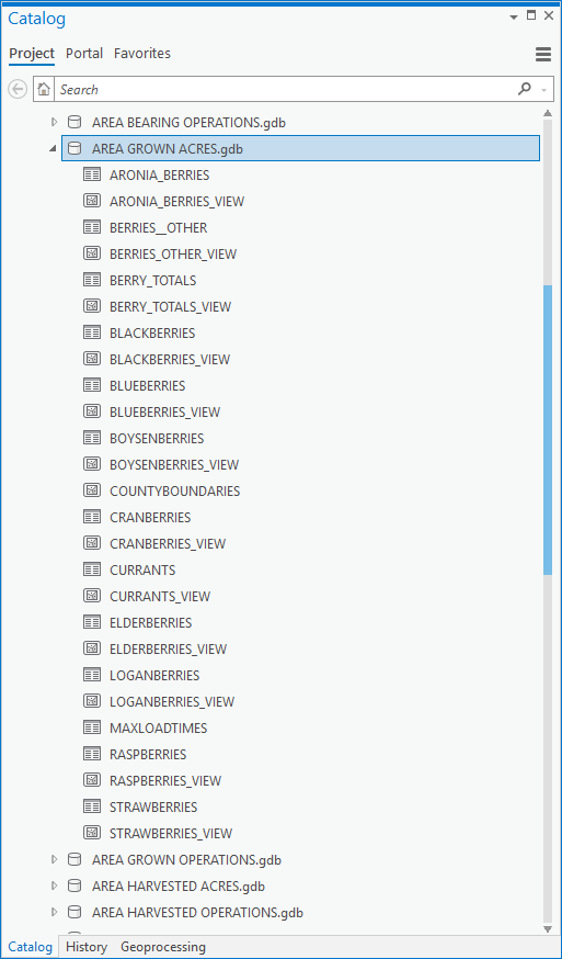
Expanding the 'AREA GROWN ACRES' dataset we can see the views, ready for use in a map:
Lets have a look at a view. I'm going with peanuts. I have never made a study of peanuts, but at least I know what they are. Working with this data I learned of crops like Escarole Endive, which I may have eaten but never knew. I like red-skinned Valencia peanuts, I think they make the best peanut butter, and to believe the packaging, excellent ones come from Texas. I also buy a lot of peanuts in the shell (roasted, unknown variety, unsalted) to feed the wildlife in our yard, and that packaging assures me Virginia peanuts are great too. Peanuts here we go.
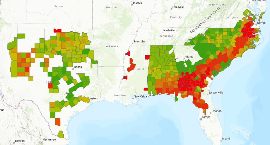
I added PEANUTS_VIEW from the workspace YIELD LB PER ACRE.gdb to my map and symbolized by VALUE with graduated color using 10 classes with a color ramp from green to red (red is high productivity). Displaying all features I can see the engine room of peanut productivity is the arc of land across Mississippi, Alabama, Georgia, the Carolinas and up to Virginia, and more west of the Mississippi in Oklahoma and Texas.
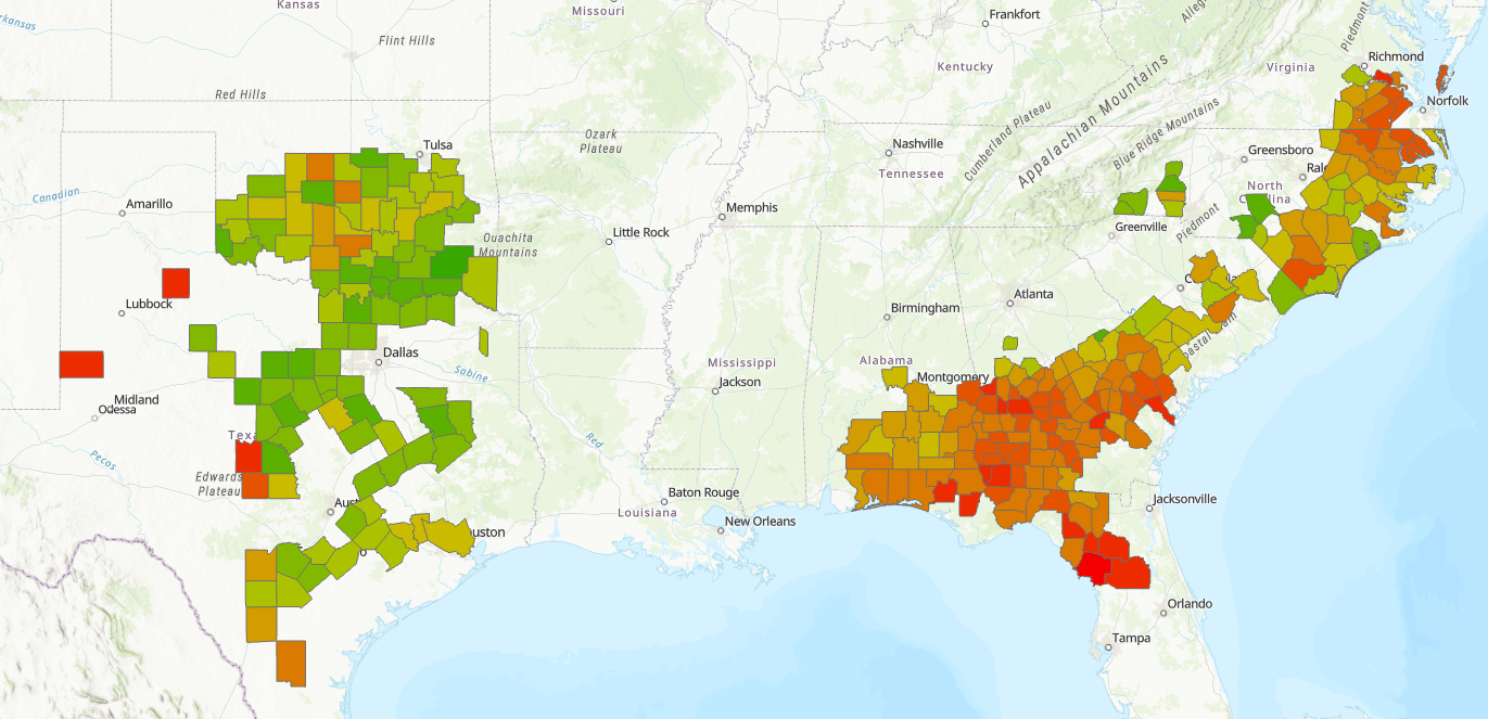
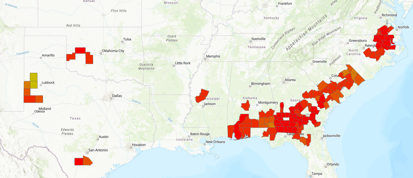
Time enabling on YEAR gives us the real story behind peanuts though. In the download, view the 30 second movie PeanutsTheMovie.mp4. This animates in single-year frames for all years 1934 to 2018.
Here is 1934, what we might now call historically low yield and only in the east of 'peanut country':
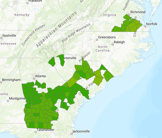
By 1965 productivity and range had increased:

By 1975 productivity and expansion had greatly increased:
..and moving right along to the current time, peanut yield per acre has reached yields ten times historic values:
A common issue with big data is you want to find what has changed - what is new. This is where the script tool ReportLoadTimes comes in. This reads each MAXLOADTIMES table and emits a message about the most recent crop(s) statistic in each workspace. For my data at time of writing I can see this:
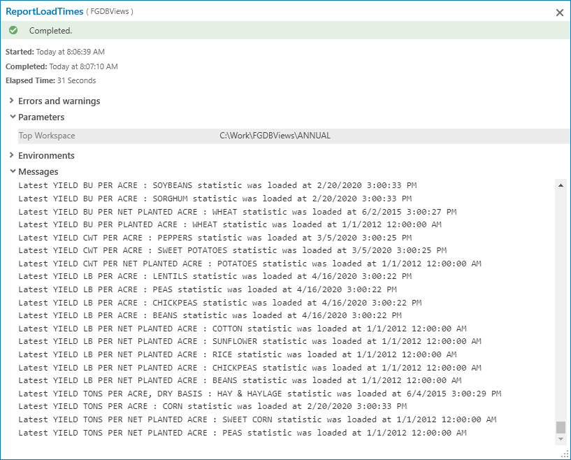
So for example in my workspace YIELD LB PER ACRE where my peanuts view lives, the latest statistics are for these crops updated a few days before finishing this blog:
Latest YIELD LB PER ACRE : LENTILS statistic was loaded at 4/16/2020 3:00:22 PM
Latest YIELD LB PER ACRE : PEAS statistic was loaded at 4/16/2020 3:00:22 PM
Latest YIELD LB PER ACRE : CHICKPEAS statistic was loaded at 4/16/2020 3:00:22 PM
Latest YIELD LB PER ACRE : BEANS statistic was loaded at 4/16/2020 3:00:22 PM
All crops sharing the latest load date are reported.
I hope this gives you confidence to tackle your own big data problems with ETL and File GDB views. I read that for NASS data there are many commercial decisions made based on crop statistics and you will have your own business drivers. Caveat: NASS has some peculiarities that prevent all records displaying, for example some VALUE values are non-numeric and are discarded by this processing, and there are some county aggregations that cannot be mapped to county boundaries, so don't go building your peanut butter factory on my analysis.
Have fun!
You must be a registered user to add a comment. If you've already registered, sign in. Otherwise, register and sign in.