- Home
- :
- All Communities
- :
- Industries
- :
- Education
- :
- Education Blog
- :
- Exploring Oceans as Regions with Geospatial Techno...
Exploring Oceans as Regions with Geospatial Technologies
- Subscribe to RSS Feed
- Mark as New
- Mark as Read
- Bookmark
- Subscribe
- Printer Friendly Page
- Report Inappropriate Content
Exploring Oceans as Regions with Spatial Technology. Nearly 71% of the world is covered by ocean. For centuries, and even often in our current era, oceans are mapped as a uniform color and are not thought of as regions, but as geographers and oceanographers are discovering, oceans are as dynamic as land—many would argue even more so—and examining oceans as regions is possible with Spatial Technology.
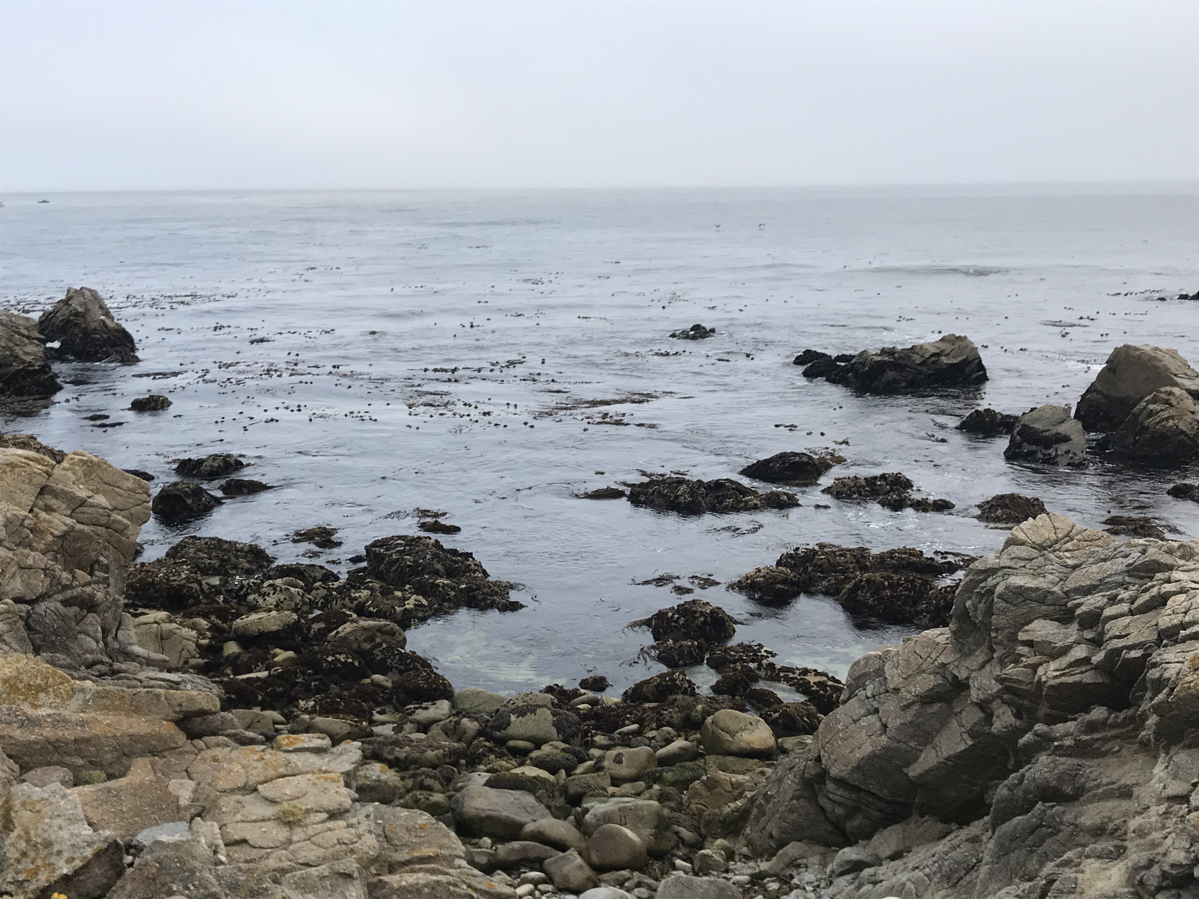
Pacific Ocean at Pacific Grove, California, photograph by Joseph Kerski.
Understanding the Ecological Marine Units data. In many respects, the oceans are the “last frontier” on Earth—much about them remains unknown and unmapped, but given the importance of oceans to the carbon cycle, the food chain, biodiversity, climate, and many other earth systems, there is a growing sense that this needs to change. Given the vastness, the changing nature, and the 3D nature of the oceans, Spatial Technology is turned to as a solution to understanding and mapping the oceans. The Ecological Marine Units (EMU) map has been created, to portray a systematic division and classification of physiographic and ecological information about features in the ocean. Part of the EMU is a 3D data model of the ocean—and 3D data visualization tools to go along with the data. A statistical clustering methodology was also developed for identifying the physiographic structure of the water column based initially on temperature, salinity, dissolved oxygen, and nutrients—i.e., the usual suspects that will likely drive ecosystem responses.
This methodology was developed by Esri’s Kevin Butler and vetted by distinguished spatial statistics professor Noel Cressie of the University of Wollongong in Australia. That information was connected to species distributions (initially from the Ocean Biogeographic Information System or OBIS), biogeographic realms, and seabed habitat and biotopes representing the response of these ecosystems to the physical setting (e.g., the biological distribution/response to ocean acidification). The Group on Earth Observations (GEO) officially commissioned the project as a means of developing a standardized, robust, and practical global ecosystems classification and map for the oceans. GEO is a consortium of almost 100 nations collaborating to build the Global Earth Observation System of Systems (GEOSS). The EMU project is seen by GEO as a key outcome of the GEO Biodiversity Observation Network (GEO BON) and the new GI-14 GEO Global Ecosystems Initiative (GECO).
For more information, examine this document: https://blogs.esri.com/esri/esri-insider/2016/03/14/new-map-sets-framework-for-describing-ocean-ecol....
Using the Ecological Marine Units as an investigative tool. Begin your investigation of the Ecological Marine Units with this Explorer map: https://livingatlas.arcgis.com/emu/ Click anywhere on the map and you will observe a graph to the right of the map with ocean water variables displayed in graph form by depth. Clicking on the Temperature Profile title of the graph yields the other graphs (nitrate, salinity, and others) available for that location.
Pan to Australia and click a point off the shore of New South Wales or Victoria; the map should look similar to that below.
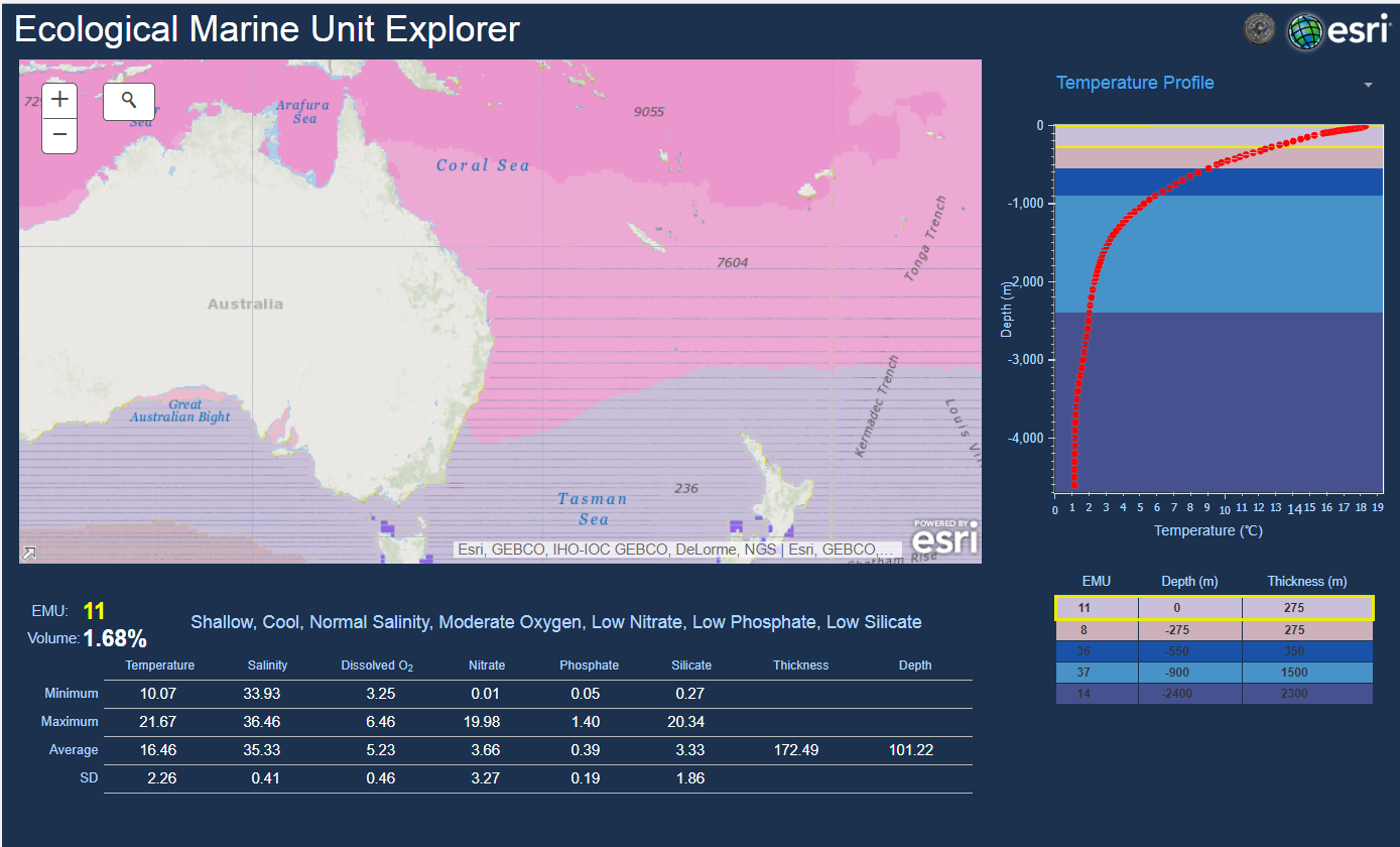
Adding to the complexity of understanding the ocean’s regions is that for any one location, the regions overlay, or more accurately, underlay each other. On land, while elevation influences the plant and animal life, climate, water, soil, and vegetation, to name a few, each location on land is represented by a single region. But in the oceans, the regions sit (or “slosh”) atop each other. Consider the example above. Off the coast of Australia lies EMU region 11—Northern and Southern Subtropical Epipelagic. Epipelagic refers to the part of the oceanic zone into which enough light penetrates for photosynthesis. At the location clicked, it is 275 meters thick. Underneath this is EMU 8 – the subAntarctic, North Atlantic, and North Pacific Epipelagic, extending another 275 meters, and underneath that is EMU 36, the Atlantic, Subantarctic, and North Pacific Subtropical Bathypelagic region. Bathypelagic – from Greek βαθύς, deep – refers to the part of the pelagic zone that extends from a depth of 1,000 to 4,000 m below the ocean surface. Here, no primary production of plant life, so all creatures that live there are carnivorous, eating each other or feeding on carcasses that sink down from above. And underneath this are EMUs 37 and 14.
For a two-dimensional cross section with these zones labeled by depth, see Figure 1 in the metadata booklet: http://www.aag.org/galleries/default-file/AAG_Marine_Ecosyst_bklt72.pdf
Examine Ecological Marine Units around the world. Use the Table on page 10-11 of the same metadata booklet http://www.aag.org/galleries/default-file/AAG_Marine_Ecosyst_bklt72.pdf (this is the same as page 6 of 19 in the PDF), and compare EMU 11 to the other EMUs in term of depth, temperature, dissolved oxygen, nitrate, phosphate, and silicate.
Examine the map on page 12-13 of http://www.aag.org/galleries/default-file/AAG_Marine_Ecosyst_bklt72.pdf (this is the same as page 7 of 19 in the PDF) and note the distribution and spatial patterns of the EMUs around the world. Which would you say is the largest in area? Be careful! EMUs 19 and 31 in the Southern Ocean may look like the largest, but remember that the map projection may distort the area of land and water near the poles.
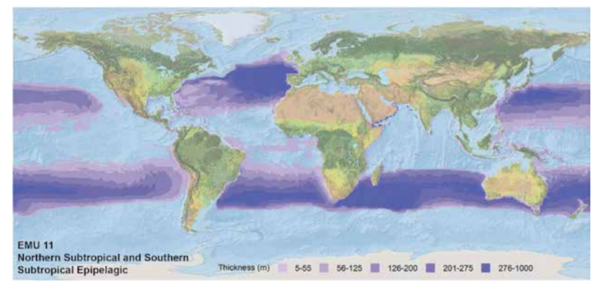
Scroll down to page 20 and 21 (page 11 of 19 in the PDF) and examine the map of EMU 11 (reproduced below) that was present at the surface off the southeast coast of Australia —the Northern and Southern Subtropical Epipelagic. How would you describe the spatial distribution of this EMU?
Note the Equatorial location of EMUs 18 and 24, and predict their mean temperature compared to other EMUs. Scroll back up to the table—was your hypothesis correct? Note the high amount of dissolved oxygen contained in EMUs 5 and 16. Knowing that cold water can hold more dissolved oxygen than warm water, predict the location of EMUs 5 and 16. Scroll back up to the map. Was your hypothesis correct?
Examine Australia EMUs. Go back to the interactive EMU map (https://livingatlas.arcgis.com/emu). Begin again by clicking off the coast of southeast Australia. Or choose another area of the world of interest to you. Gradually move and click northward along the east coast, observing the graph at the right. What do you notice about the water temperature as you move north? Why? How and why does the dissolved oxygen change?
Always be critical of the data—EMUs being no exception. Go Again, keeping with our theme of being critical of the data, there is no water quality measurement buoy or set of ships at every square meter on the surface of the ocean with a tether extending down to the ocean floor. Rather, the data are sampled as follows:
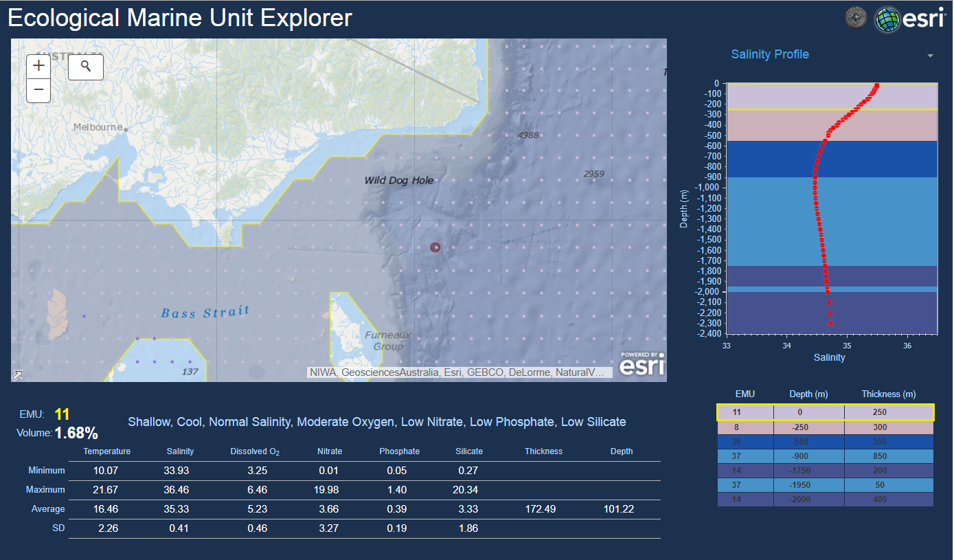
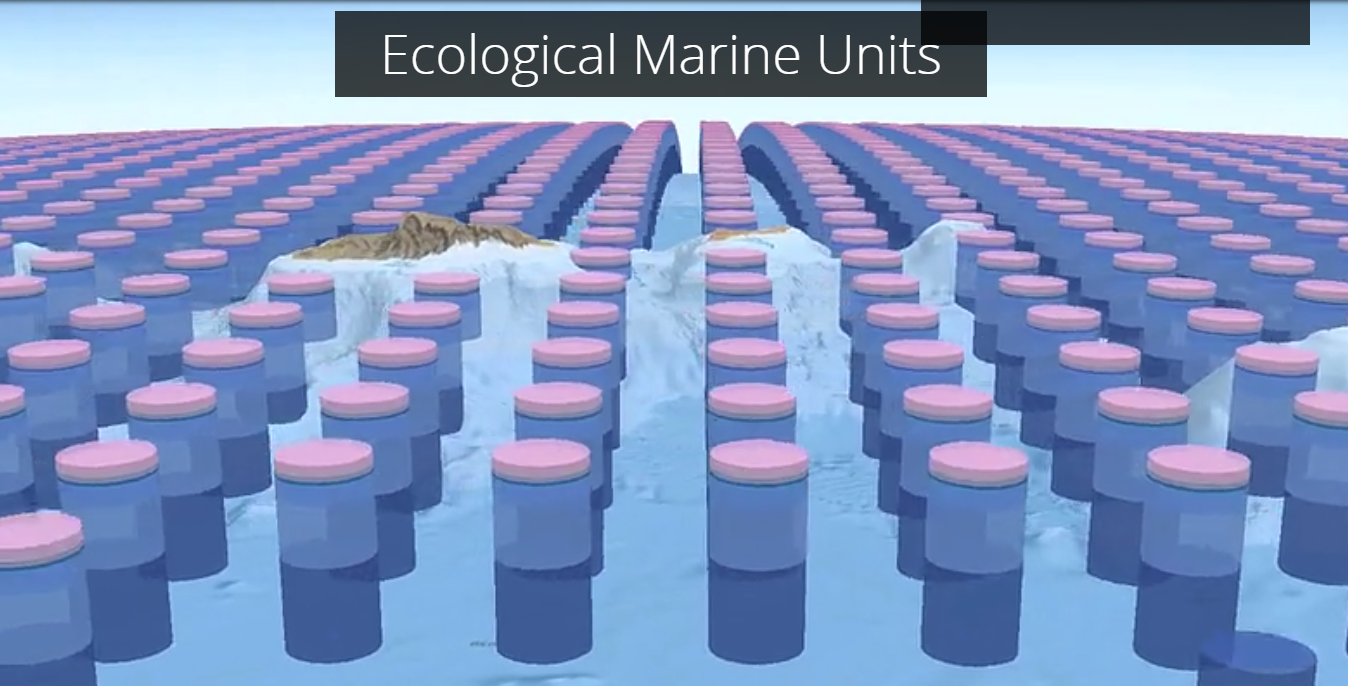
The fundamental approach undertaken was to stratify the ocean into physically and chemically distinct areas. The stratification was produced from unsupervised statistical clustering of data from NOAA’s 2013 World Ocean Atlas version 2. The data used in the clustering represent 57-year average values for temperature, salinity, dissolved oxygen, nitrate, phosphate, and silicate. Approximately 52 million ocean data points representing the entire water column. The horizontal resolution of the data is ¼°, or approximately 27 km near the equator. The depth intervals are variable from 5 m near the surface to 100 m in the deeper regions (>2000 m) for a total of 102 depth levels. The EMUs were produced from a k-means statistical clustering of the point data, resulting in 37 distinct clusters. Each cluster, or EMU, is a physically and chemically distinct volumetric region. Thus, the data was rigorously produced, but zoom in until you see the data points, as shown below. You can now see the data points spaced at ¼° (one quarter of a degree of latitude and longitude) apart. In the same way on land, you examined a sample grid of data points from the Degree Confluence Project to examine physical and cultural regions.
Dig Deeper with EMUs. Go To dig deeper, literally, examine some of the 3D views in this story map of the EMUs. Scroll down to “Additional Examples” at the end and examine the areas offshore from Ireland and offshore from Central America. This might provide a better sense of the 3D nature of each “column” of data across the ocean.
Skim this research document to discover how the EMU data can be used by those using Spatial Technology: https://www.esri.com/en-us/about/science/ecological-marine-units/research/. To examine the data in 3D in a Spatial Technology environment requires the use of a desktop GIS called ArcGIS Pro. Good news! With your ArcGIS school account, you can also get access to ArcGIS Pro.
You must be a registered user to add a comment. If you've already registered, sign in. Otherwise, register and sign in.
-
Administration
38 -
Announcements
44 -
Career & Tech Ed
1 -
Curriculum-Learning Resources
178 -
Education Facilities
24 -
Events
47 -
GeoInquiries
1 -
Higher Education
518 -
Informal Education
265 -
Licensing Best Practices
46 -
National Geographic MapMaker
10 -
Pedagogy and Education Theory
187 -
Schools (K - 12)
282 -
Schools (K-12)
184 -
Spatial data
24 -
STEM
3 -
Students - Higher Education
231 -
Students - K-12 Schools
85 -
Success Stories
22 -
TeacherDesk
1 -
Tech Tips
83
- « Previous
- Next »